Journal of Defense Management
Open Access
ISSN: 2167-0374
ISSN: 2167-0374
Research Article - (2022)Volume 12, Issue 3
One of the decisive factors for victory in military operations is the performance of the weapons system. This is reflected in the Required Operational Capabilities (ROC). ROC is determined in the acquisition planning phase when the quantitative goals of the weapon system are clarified. Inaccurate ROCs can generate serious consequences, such as failures in testing and evaluation, increases in lifecycle costs, delays in the acquisition, and, in the worst case, suspension of the acquisition project. In this research, we propose a novel framework for determining ROC by the combination of optimization and simulation techniques. First of all, an optimization model is formulated to maximize the mission success rate, taking into account the performance and effectiveness of the acquiring weapon system. For the optimization modeling, we generated a set of equations while figuring out the relation between the Measure of Performance (MOP) and the Measure of Effectiveness (MOE) by inspecting observed data from the simulation run. We describe relevant techniques and experiments that were performed to demonstrate our methodology has real world applicability to the Defense Acquisition Process.
Required operational capabilities; Measure of performance; Measure of effectiveness; Defense acquisition process; OneSAF wargame model
One of the most important decisions to be made in securing required combat capability is determining the Required Operational Capabilities (ROC). The ROC, a standard step in the defense acquisition process, is a list of requirements of the weapon system. Settling on an ROC involves two essential tasks-identifying a desired outcome and quantifying the conceptual demands. If the weapon system of interest is an assault rifle, for example, one desired outcome could be rifle can hit a target from a distance and be quickly reloaded. To quantify the corresponding conceptual demands, one could propose the rifle range is greater than 450 meters, and reloading time is less than 10 seconds. It is important that each decision be determined by different groups. Military personnel, for instance, should be in charge of the first task and engineers in charge of the second. Thus, the correct understanding of military needs and the transformation of those into quantifiable items are equally important parts of the process. A Ministry of National Defense (MND), also known as a Department of Defense, defines ROC across all phases of the acquisition process followed by the System Engineering (SE) philosophy. In spite of the SE aid, it is still hard to find an efficient and effective way of defining ROC. For example, Table 1 shows some ROC items, along with its numerical criteria, and an explanation of why those criteria are defined. Suppose we want to develop or purchase a counter-artillery missile system with the goal of a target interception rate of higher than 95%. How can we establish a numerical criterion for other elements of ROC? What is the exact number for this? How do we know the relation between the maximum speed of the missile and the interception rate? Indeed, the interception rate might be the function of other ROC items. Moreover, a set of combinations that accomplishes the goal may not be unique. For instance, one combination of ROC capable of attaining a 95% interception rate could include an effective range (4 km), a maximum speed (Mach 1.0), and a launch interval (1 per minute). In such a case, the criteria described in Table 1 are unnecessarily over defined. In the real-world, this is very common. After all, the perspective of an engineer is quite different from that of military personnel. In the view of an engineer, as long as the system can intercept the enemy missile with 95% interception rate, they think the other ROCs can be determined on their own. However, the military wants to define the criteria of all sub-systems from the perspectives of users and owners. The challenges mentioned above force the MND, when determining the numerical criteria of ROC, to refer to the criteria of a benchmarking system (e.g., system successfully deployed on the market). Such decision making, however, forces the MND to spend time and money, unnecessarily, developing a system. Otherwise, the MND decides, based on sensitivity analysis, the criterion of each ROC item separately. However, the induced solution may be optimal for each component, but it may not be a universally optimized solution. In this work, we study a framework for determining ROC with a mathematical optimization model supported by a simulation model. In section 2, we review previous works and describe the contribution of our work. In section 3, we propose the framework for determining ROC, including a detailed description of the mathematical model. In section 4, we introduce a detailed study example to help the reader understand how the proposed framework is applied in the real world. Lastly, we explain the limitation of the research as well as suggestions for further study.
| ROC item | Numerical criteria | Reason |
|---|---|---|
| Effective range | 5 km | refer to benchmarking system |
| Maximum speed | Mach 1.0 | refer to benchmarking system |
| Launch interval | 2 per min | refer to benchmarking system |
| Interception rate | 95% | objective of MND |
Table 1: ROC example: Counter-artillery missile system.
In national security, a critical process in generating military capacity is defense acquisition. Decision makers can decide on defense acquisition generally by using the following three techniques: cost-effectiveness analysis, cost-benefit analysis, and simulationbased acquisition [1]. The traditional approach most commonly used in defense acquisition is Cost-Effectiveness Analysis (CEA). CEA is used to secure the maximum effect at the minimum cost. Because “effects” are evaluated in terms of ratios rather than monetary values, it is possible to make relative comparisons between alternatives. However, the measures and judgments of the alternatives themselves are limited. CEA is primarily used for the analysis of strategic effectiveness in terms of System of Systems (SoS) but does not provide individual logic for each system [2,3]. Another popular method of analysis is cost-benefit analysis (CBA). CBA and CEA have many similarities. The main difference is that CBA must value every outcome in terms of economics while CEA prioritizes alternative spending without having to evaluate the dollar value of the system. CEA is used in strategic decision-making of defense acquisition because it is difficult to estimate the number of benefits from weapon systems if the benefits of the system acquisition are measured in monetary units rather than ratios. In addition, the benefit estimates of weapon systems between peacetime and wartime concepts are not rational. So, when quantifying benefits, decision makers prefer to use CEA to CBA [4,5].The third large decision supporting tool to determine ROC is Simulation-Based Acquisition (SBA). The U.S. Department of Defense (DoD) defined SBA as an acquisition process that enables DoD and industry to use powerful and collaborative simulation technology integrated into acqui- sition stages and programs. This means that the SBA can substantially reduce the time, resources and risks of weapon system acquisition. It does so by using, throughout the entire process, Modeling and Simulation (MS), including analysis and determination of weapon system requirements, analysis/ design, production, testing/evaluation, training, operation, and logistics support [6-8].To derive optimal capabilities, decision makers should systematically analyze the various alter- natives presented at the strategic level of defense acquisition. As a result, the specifications and required capabilities of weapon systems and equipment to be used must be developed as ROC. Bulgaria, as a member of NATO, developed a prioritization methodology using the Analytical Hierarchy Process (AHP) for the development of ROC [9]. In capability development processes, South Africa proposed a five-step capability decomposition approach to integrating operational needs and system requirements [10]. To manned and unmanned aerial vehicles, Canada introduced the Hierarchical Prioritization Capabilities (HPC) method. This method provided the link between mission requirements and capability delivery options. This approach eliminates the need to com- pare all possible role and task pairs of UAVs required for AHP [11]. A review of the literature reveals that researchers have conducted studies on defense acquisition decisions at the strategic level, on operational capability prioritization through multi-criteria decision making, and on coming up with capability development processes. Researchers have not, however, come up with a mathematical framework to determine the optimal ROCs that take into account system performance and effectiveness. To the best of our knowledge, there is a lack of research focusing on the use of simulation and optimization together to determine ROCs; nonetheless, there many studies to use simulation models to analyze combat effectiveness in this article then, we study a novel framework to support such a determination. Contributions of this paper are highlighted as follows-
• A novel ROC determination concept and framework has been suggested by the combination of optimization and simulation techniques. The research investigates a detailed process for determining required operational capabilities from beginning to end. The process draws a clear distinction between the military personnel’s and the engineers’ responsibilities.
• This work develops a mathematical optimization model that takes into account the performance and effectiveness of the acquiring weapon system while maximizing the mission success rate.
• This work derives a series of constraints of the proposed optimization model by inducing, with the support of a simulation model, the relation between the MOP and the MOE. This is the first use of a simulation model, especially a war-game model, to define equations used to construct the mathematical model. We describe specific techniques as well as relevant issues derived from this non-trivial process.
In this section, we first describe the general framework for determining ROC elements and investigate the mathematical optimization model for implementing the idea. The whole process of the framework is described in Figure 1. In the sections that follow, we detail each step.
Overall process
Mission statement and MOE: The first step is to define a mission that must be accomplished by acquiring a system of interest. As the definition affects the entire ROC decision-making process, it should be precise. One could define, for example, the following-
• The number of casualties in the course of reconnaissance operations is decreased by 10%.
• The enemy detection capability should be significantly enhanced.
In the first example; the military explicitly defines the goal of the system using the exact number. However, as stated in the second example, the goal can be defined ambiguously as well. As the mathematical model consists of the explicit form of a set of variables, we draw out quantifiable elements from the statement above, called MOE. In this research, we assume MOE and combat effectiveness [12] to be the same. Possible MOEs induced by the second statement above may include the number of detection, range of sensor, the probability of successive detection, and so on. The first step could necessarily involve the abstraction and simplification of the real-world.
Definition of MOP: MOEs are a simplified and quantified representation of the goal of the mission. However, most ROC items and MOEs are not identical because the specification of a weapon system mostly consists of a set of components defined from an engineering perspective. In Table 1, for instance, Effective Range or Maximum Speed explains the performance of the weapon system, not exactly the effectiveness of the system, also known as MOP. As explained in Figure 1, ROC is usually a subset of MOPs. As we already define the mission success by using some MOEs in the first step of the framework, and we note that MOPs define the ROC, we now need to define the relationship between MOPs and MOEs
Definition of the relation between MOPs and MOEs: In our framework, we assume that there exists an oracle function in which it takes MOPs as its input value and returns MOEs as the output of the function. Such an oracle function can be defined in an empirical way by conducting numerous experiments. One could estimate, for example, the probability of successive detection (i.e. MOE) by performing real-world experiments with different settings of Range of Sensors (i.e. MOP). In most cases, though, such experiments are limited for the following reasons. First, we do not have confidence in which MOPs would account for the result of MOEs. This complicates the design of experiments. Second, realworld experiment (called field experiment) involves a risk when it comes to a real battlefield situation. Third, even though we figure out valid MOPs that affect the result of MOEs and find a way to conduct experiments, it could be quite costly. Lastly, determination and confirmation of ROC ought to be concluded before the weapon system is actually developed. It is not reasonable to propose the goal of the system after it is already built. For these reasons, we suggest using the simulation model as our oracle function. We take advantage of simulation models such as low cost, repetitiveness, and low risk. Most importantly, the simulation model can provide us a logical basis for the relation between MOPs and MOEs.
Formulation of optimization model: Our aim with this framework is to find the proper number of ROCs, a subset of MOPs, with which we want to contribute to mission success. To quantitatively express the qualitative factors of mission success, one should express them in the explicit form of MOEs. The problem we are looking for is to maximize or minimize MOE. If MOE has a positive impact on mission success, it should be maximized; if it has a negative impact, it should be minimized. As shown in Figure 1, there are other real-world considerations environmental aspects. The most representative consideration is the cost of the weapon system. Another consideration could be the technical readiness regarding the proposed system. Such factors are applied to the model as constraints. In later sections, we detail the mathematical expressions of our model.

Figure 1: General framework overview for determining ROC elements by mathematical optimization.
Optimization model
Let X is be a set of MOPs. For example, possible X can be X={velocity, weight, range of rifle}. Let Y be a set of MOEs. For example, Y={number of death, probability of success on task}. We define real-valued vector x and y where xi takes the value of MOP i∈X and yi takes value of MOE i∈Y. Let z(y) ∈ R be a function that can be used as the surrogate of mission success. If z(y) is properly defined, then we want z(y) to be maximized. Given the difficulty of quantifying the mission success, z(y) may not be formally defined. In order to define z(y) we first categorize the vector y using the following criterion. The mission is likely to succeed as:
• yi increases (decrease)
• yi has no effect
• li ≤ yi ≤ ui
• yi relation is not known
The criterion above is exhaustive and mutually exclusive of realworld considerations. Moreover, classification is intuitively easy for military personnel who are responsible for the job. We define subset Yj ⊆ Y to be a set of MOE that falls into the jth category above. We assume Y1 ∪ Y2 ∪ Y3 ∪ Y4=Y where each set are mutually exclusive. In this case, our optimization problem can be defined as-
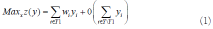


Since our objective is to find a vector x that maximizes mission success, yj∈Y1 is composing the objective function with a corresponding weight vector wj. Other yj∈Y \Y1either does not affect mission success or relation is not defined, hence, such terms are multiplied by 0. The objective function z(y) is linear on y but not possible on x. Because we assume that there exists an oracle function f(x) → y, we define the relation between x and y (i.e. equation 3). A set of inequalities (4) defines the relation between MOPs. Inequalities (5) refer to constraints representing the environmental aspects of the system. For example, typical constraints for these inequalities should be a system’s cost limitation.
One of the common challenges is predicting cost [13]. If we have sufficient data for estimating the Cost Estimating Relationship (CER), we can use it in relation to inequalities (5). Or we can obtain cost information on the specific performance value and estimate an unknown cost by the interpolation. For example, Figure 2 shows us the situation where we do not have perfect information on the cost of xj, certain MOP, but have three reference points. Each reference point has a cost (i.e. ci) and corresponding value of MOP (i.e. ei). One may acquire reference information by conducting some statistical analysis or simply referring to the benchmarking weapon system. The cost of xj can then be estimated by interpolation as described in equation (6) and mathematical expressions for implementing this logic are equations (7-11) where MOP j has Rj reference points.

Figure 2: Example on approximation of cost as a piece-wise linear functions.
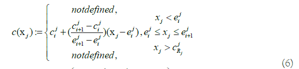
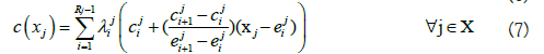
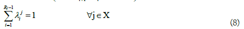


Where lj and uj represents the lower and upper bound of MOP xj. The binary variable λj defined to have 1 if we choose reference interval starting from point i. A weapon system is composed of many sub-systems that interact with each other. The proper analysis of it may require elaborate mathematical expression. For instance, Figure 3 describes two MOPs (i.e. xA, xB) being used to define the relation to MOE yC. In the upper part of the figure, the r elation between two MOPs and MOE is defined as h(x)=yC. However, in typical oracle function, any simulation model in our research, may miss out on embedding a property of the system. Let’s assume that the system, as shown in the lower part of Figure 3, has a serial structure for which any one of the system components fail. The entire system should be defined with a different expression, g(x)=yC. In the real world, such a case occurs commonly. For instance, xA could be the MOP indicating the performance for the fire control radar system and xB could be the MOP representing the performance of the engagement system. Since engagement is only initiated after the radar detects the target, the weapon system clearly has the serial structure. One of the possible mathematical expressions for the detailed study is given below. First, we define binary variables indicating the break event of system j.

Figure 3: Example on necessity of if-then constraints.
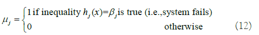
We define an additional indicator variable γ ∈ {0, 1} that takes 1 if all subsystems work and 0 if any one of the subsystems fails. And a set of inequalities that follows defines the aforementioned logic.


Inequalities (13-19) may be neither unique mathematical expressions for the case nor the most efficient way for describing the logic. Still, the critical point we want to highlight here is that we have easy access to represent a real-world complex with the mathematical model we are using.
To demonstrate how the proposed framework operates, we conducted an experiment on an Unmanned Ground Vehicle (UGV) system. UGV systems conduct operations without an onboard combatant presence. As the system has complex components such as sensors, control systems, and guidance interface, we can induce many corresponding MOPs. For experimental purposes, we selected 5 MOPs and 3 MOEs, as described in Table 2. In the last column, we describe the level of each MOP, different factor values for designing experiments. For example, Range of Detection (RD) has 3 levels 100 meters, 500 meters, and 1,000 meters. Issues regarding the design of experiments are not of interest in this work, so discussions on the selection of MOP and levels are not relevant. For the description of an optimization model, we define a mathematical ingredient first.
Let X = {VE,RD,TP,AR,RR} be a set of MOPs. Let Y = {TD,DF,DH} be a set of MOEs. Let xi ∀i ∈ X be the value of MOP and yi ∀i ∈ Y be the value of MOE. Assume that all MOEs fall into the first category described in previous section where yTD and yDH are positively correlated with mission success and yDF is negatively correlated. This process should be done by military personnel. The next step is to find the explicit form of the relations between MOPs and MOEs. We require, as discussed earlier, the oracle function. For the analysis, we chose One Semi-Automated Forces (One SAF) war-game model (version 6.01, international edition). One SAF is a composable simulation architecture that supports both Computer Generated Forces (CGF) and Semi-Automated Forces (SAF) operations and has been used in multiple Army Modeling and Simulation domain applications worldwide [14]. The following assumptions (scenario) were made for the experiments. Figure 4 shows an image capture of the experiments.

Figure 4: One SAF simulation environments: UGV reconnaissance.
• A BLUE force (reconnaissance team) consists of 4 UGVs, 3 infantry combatants, and 1 command and control vehicle.
• A RED force consists of 4 anti-tank teams. Each team is armed with an anti-tank rocket.
• Area of operations is 25 km × 25 km
| Code | Description | Level |
|---|---|---|
| MOP | ||
| VE | height of vertical extender (meter) | {1, 20} |
| RD | range of detection (meter) | {100, 500, 1000} |
| TP | transmission power (dBm) | {10, 40} |
| AR | accuracy rate of RCWS* | {0.5, 1.0, 1.5} |
| RR | range of RCWS (meter) | {400, 850, 1300} |
| MOE | ||
| TD | number of targets detected | ∈Z |
| DF | damage of BLUE force (%) | ∈R |
| DH | damage of RED force (%) | ∈R |
Note: *Remote Controlled Weapon Station (RCWS)
Table 2: List of MOPs and MOEs for UGV.
We performed 108 experiments (i.e. 108=22 × 33). Each experiment included 20 replications and data on the explanatory variables were collected. Given in Table 3 are the ANOVA test results showing whether there was a significant difference between response (i.e. MOE) and explanatory variables (i.e. MOP). It turned out that MOP RD explains well all the MOEs, while AR and RR failed to account for MOEs. Based on the belief that a statistical relationship can establish a deterministic expression, we conduct the multiple regression analysis by using MOP data as the explanatory variable and MOE as the response variable. Regression analysis results of MOE TD, DF, and DH are given in Tables 4-6 respectively. In Table 4, two explanatory variables (i.e. RD, TP) were selected as the result of stepwise regressions where adjusted R2 value was 74%. We interpret the regression model to be statistically significant based on the F-test result. Now, the 2 variable linear multiple regression models can be written as
TD=2.445+0.013 × RD− 0.038 × TP (20)
| Response | VE | RD | TP | AR | RR |
|---|---|---|---|---|---|
| TD | 0.847 | <0.001 | 0.283 | 0.9 | 0.925 |
| DF | 0.707 | <0.001 | <0.001 | 0.614 | 0.559 |
| DH | 0.196 | <0.001 | <0.004 | 0.915 | 0.938 |
Table 3: T-test and ANOVA results for explanatory variables.
| Explanatory variable | Estimate | Standard error | t value | p value |
|---|---|---|---|---|
| Intercept | 2.445 | 0.648 | 3.771 | 0.000*** |
| RD | 0.013 | 0.0007 | 17.362 | 0.000*** |
| TP | -0.038 | 0.018 | -2.112 | 0.037* |
Note: F(2,105)=152.9, p-value: 0.000***, adjusted R2: 0.7396, ***p<0.001, *p<0.05
Table 4: Regression result for response variable TD.
| Explanatory variable | Estimate | Standard error | t-value | p-value |
|---|---|---|---|---|
| Intercept | 3.591 | 0.183 | 19.602 | 0.000*** |
| RD | -0.0009 | 0.0001 | -5.765 | 0.000*** |
| TP | -0.0265 | 0.0036 | -7.283 | 0.000*** |
| RR | -0.0002 | 0.0001 | -1.452 | 0.15 |
Note: F(3,104)=29.46, p-value: 0.000***, adjusted R2: 0.4438, ***p< 0.001
Table 5: Regression result for response variable DF.
| Explanatory variable | Estimate | Standard error | t-value | p-value |
|---|---|---|---|---|
| intercept | 2.937 | 0.4883 | 6.016 | 0.000*** |
| VE | -0.0302 | 0.0192 | -1.566 | 0.12 |
| RD | 0.0028 | 0.0005 | 5.662 | 0.000*** |
| TP | -0.0512 | 0.0122 | -4.193 | 0.000*** |
Note: F(3,104)=17.37, p-value: 0.000***, adjusted R2: 0.3145, ***p< 0.001
Table 6: Regression result for response variable DH.
Similarly, we obtain the regression model for MOE DF and DH
based on the result in Tables 5 and 6. As discussed in previous section,
cost information plays a role in the model as a constraint. In this
detailed study example, all cost information was manipulated.
We assume that MOP j ∈ X has Bj numbers of reference points
where break point i ∈ Bj defines cost and corresponding MOP
value  . For instance, if transmission power in Table 2 costs 50 units
(where its level is 10) and 200 units (where the level is 40) then
. For instance, if transmission power in Table 2 costs 50 units
(where its level is 10) and 200 units (where the level is 40) then  =50,
=50, =10 and
  =200,
=200,  =40. The values of parameters that we assumed are described in Table 7. We
additionally define binary variable
=40. The values of parameters that we assumed are described in Table 7. We
additionally define binary variable  as we discussed in previous section.
Then, the resulting optimization model is as follows-
as we discussed in previous section.
Then, the resulting optimization model is as follows-


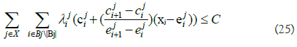
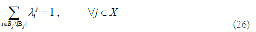


where C in (25) is the budget constant of the system and wi is the weight value of MOE i. The weight vector could be defined in multiple ways. It could be importance of MOE if decision maker want to place a difference between MOE. Or the decision maker could make the weight vector credibility of the equation. In our model, the weight value we use in Tables 4-6 is adjusted R2 value of MOE variable. Inequality (29) represents the relation between MOPs, explaining the fact that RCWS can engage the enemy only if it is only the radar that detects the enemy. In the general model, this falls into category (4). An optimization model is implemented and solved using GAMS 30.3.0 with BARON 19.12.7 Solver. As we have an arbitrary cost in the detailed study, an exact solution and its optimal objective value to the model may be unimportant. However, we have some interesting observations. Figure 5 shows the dynamics of optimal MOE value, called yi, with a different choice of the whole budget (i.e. a constant C in the model). The horizontal axis represents the proportion of the parametrized budget to the maximal budget, where the maximal value is defined to cover the cost where every MOP has its upper bound level. On the rightmost of the graph, for instance, we consider having sufficient budget. The cost value of 0.5 means that we have 50% of the budget to the maximal number. The vertical axis represents the value of MOE. Given the condition that we have sufficient budget, the optimal solution is y*=(y*TD, y*DF, y*DH)=(15.06, 2.22, 5.19). If the budget decreases, then y*TD, y*DH decreases but y*DF increases. For example, when a budget is 35% of the maximal, we have y*=(11.81, 2.57, 4.49). This is a reasonable result in the sense, on a small budget, the weapon system is poor. Therefore, the number of targets detected (i.e. yTD) and damage of RED force (i.e. yDH) decreases but damage of BLUE force (i.e. yDH) increases. We notice, though, a strange observation in Figure 5 in which the optimal solution is unchanged for some intervals (i.e. 0.5− 1.0 in horizontal axis). This is unreasonable as a fairly small budget could yield a similar performance of the weapon system. This issue is caused by unused explanatory variables. In our model, xAR was never used in the regression equation. As a budget decreases, the model naturally decreases the value of xAR so as to reduce the cost but not affect the objective function. In this case, we can fix such a variable to a desirable number by adding a bound constraint to the optimization model. In the research, we induce the relation between MOP and MOE by inspecting observed data from the simulation run. As interpreting the data statistically may not be unique, we may have several explicit forms of the relation. For instance, in our optimization model, equations (22-24) are all linear on x and could return a corner point solution that is trivial. For example, a solution where we have enough budget in Figure 5 is x*=(xVE, xRD, xTP, xAR, xRR)=(1, 1000, 10, 1.0, 1000) in which most of optimal values are at their lower or upper bound. However, such linear relation cannot explain some important features of the real-world such as the diminishing returns property of effectiveness [13]. Figure 6 shows the relationship between MOP xRD and MOE yTD. Based on the observed data, the relationship exhibits a diminishing property. In the figure, the solid line shows a secondorder polynomial fit and two dotted lines show evaluated values of equation (22) where we fix another explanatory variable to its lower and upper bound. Because our approach is based on multivariate regression, it is not directly applicable to use the polynomial equation rather than the linear equation. Moreover, it is beyond the scope of this research to discuss the statistical approach to dealing with diminishing effects. We would emphasize, though, that when we construct the relation between MOP and MOE we should consider not only the regression error of the estimate but also the validity of the model.

Figure 5: Dynamics of optimal MOE value with different choice of budget. 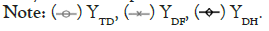

Figure 6: MOP and MOE relation with different polynomial fitting. 

| MOP | Cost | MOP value |
|---|---|---|
| VE |  =50, =50,  =200 =200 |
 =1, =1,  =20 =20 |
| RD |  =50, =50,  =100, =100, =200 =200 |
 =100, =100,  =500, =500,  =1000 =1000 |
| TP | =50,=200 |
=10,=40 |
| AR |  =50, =50,  =100, =100,  =200 =200 |
 =0.5, =0.5,  =1.0, =1.0,  =1.5 =1.5 |
| RR |  = 50, = 50,  = 100, = 100,  =200 =200 |
 =400, =400,  =850, =850,  =1300 =1300 |
Table 7: List of parameter used for cost definition.
There are two areas where the stochastic elements affect the proposed framework. The first one is in the simulation model as an oracle function. To control the randomness imposed in the simulation model, each experimental value is set as a representative value for 20 replicates as described in the detailed study. The second is in the composition of scenarios. It is recommended to test the performance of a weapon system by assuming a sufficiently large number of scenarios. As the primary focus of this research is on proposing a novel framework for ROC determinations establishing the relationship between MOE and MOP, we analyzed the case with a single scenario. However in our extended study, we may consider creating a scenario pool by varying blue/red teams’ compositions and terrain conditions. In this section, we have investigated the practical application process for our framework. Previous studies such as CEA and CBA focus on analyzing the effectiveness of weapon systems by simulation approaches. As these simulation approaches are kinds of sensitivity analysis, the detailed performance of MOPs must input as parameter values. Assuming that the UGV ROC analyzed in this study is determined by simulation, the MOE value would have been observed while changing VE, RD, TP, AR, and RR of UGVs. After then, the MOP value that presents the highest MOE value is selected as the best alternative regardless of the number of experiments. While a simulation approach only points to the best possible solution from a number of pre-determined scenarios, on the other hand, optimization approach identifies a global optimal solution from an infinite feasible space that MOP can have. From this perspective, our proposed framework can obtain the truly best ROC value by incorporating the insight provided by simulation together with optimization approach. The optimization model we discussed in this section is an example of our methodologies made real. Taking into account the complexities of real-world problems, the model can have a large number of inequalities with dozens of MOPs and MOEs.
In this research, we have described a new framework for determining ROC, which are quantified criteria of the performance of the weapon system. The framework may be summarized as follows. First, the users of the system, generally the military personnel, define a mission and extract critical elements that may influence to mission success named as MOE. Second, we categorize MOE into four mutually exclusive criteria and construct the objective function of a proposed optimization model regarding the relationship of each MOE and mission success. Third, we define connections between MOE and MOP, which are the numeric descriptions of the weapon system’s components. To find the explicit form of the relation, we run the simulation model. Various experiments and statistical analysis are required for the process. Finally, we express, as a set of constraints, the necessary environmental considerations in the real world. We discuss the limitations of the research and the corresponding direction of further research areas.
• The optimal solution solely depends on the explicit form of the relation between MOPs and MOEs. Therefore, the validity and the applicability of the model are in control of the validity and credibility of the simulation model. We cannot overstate the importance of choosing the right simulation model.
• It is essential to establish an experiment environment to conduct massive simulation runs. The deatiled study example described in section 4 deals with only one combat scenario. For a robust solution, decision makers must consider numerous scenarios. The obstacle to conducting massive experiments is the complex interface of the simulation model. For instance, in order for the MOP xRD to have level 100, we must set 5 engineering level parameters, such as sensor resolution data, contrast ratio per spatial frequency, and so on. All this is done manually. It is thus necessary to have a wrapping tool that controls the simulation model from the outside.
Regardless of the aforementioned limitations, we believe that the proposed framework is promising as we expect to have a more sophisticated war-game model in the future that leads to a trend of applying simulation-based acquisition more frequently. Moreover, our methodology provides an exact solution that meets both performance requirements and environmental considerations based on an optimization approach. The flexibility of a mathematical model will fulfill the need for changes in environments and reflection of realistic features.
The authors acknowledge financial support from the project UE192020ID funded by the Agency for Defense Development.
Citation: Cho N, Moon H, Cho J, Han S, Pyun J (2022) A Framework for Determining Required Operational Capabilities: A Combined Optimization and Simulation Approach.J Defense Manag. 12:234.
Received: 29-Apr-2022, Manuscript No. JDFM-22-17533; Editor assigned: 02-May-2022, Pre QC No. JDFM-22-17533 (PQ); Reviewed: 17-May-2022, QC No. JDFM-22-17533; Revised: 24-May-2022, Manuscript No. JDFM-22-17533 (R); Published: 31-May-2022 , DOI: 10.35248/2167-0374.22.12.234
Copyright: © 2022 Cho N, et al. This is an open-access article distributed under the terms of the Creative Commons Attribution License, which permits unrestricted use, distribution, and reproduction in any medium, provided the original author and source are credited.