Journal of Chromatography & Separation Techniques
Open Access
ISSN: 2157-7064
ISSN: 2157-7064
Research Article - (2015) Volume 6, Issue 7
Gene Expression Programming (GEP) is a novel genetic algorithm, a highly effective, stable random searching method. We take GEP to make models of Quantitative Structure-Retention Relationship (QSRR) for a series of oxygen-containing organic compounds of GC retention index, and compare the predictive results with Artificial Neural Network (ANN) and Multiple Linear Regression (MLR). The correlation coefficient on OV-1 column is 0.9919, 0.9891 and 0.9911 for GEP, ANN and MLR respectively, on SE-54 column is 0.9955, 0.9892, and 0.9917. It is shown that the predicted results by GEP are in good agreement with experimental ones, better than those of ANN and MLR.
Keywords: Gene Expression Programming (GEP); Oxygencontaining organic compounds; Artificial Neural Network (ANN); Quantitative Structure-Retention Relationship (QSRR)
Chromatography in itself is not an accurate analytical technique, but rather a separation one. The identification of oxygencontaining organic compounds can be made with the method of gas chromatographic peak in comparison with that of a standard sample of each compound. Because samples of pure compounds are not always available, it is important to develop QSRR that can efficiently predict retention parameters by using theoretical descriptors computed from chemical structure.
Quantitative Structure-Retention Relationships (QSRR) [1] establish the relationship between a chemical structure and its chromatographic retention value, which has been demonstrated to be a powerful tool for the investigation of chromatographic parameters. The main advantage of QSRR is the ability to distinguish in quantitative theoretical terms, packing materials of different chemical nature of the organic ligand and/or organic or inorganic support [2], Furthermore, it can be of valuable assistance in the prognosis of the behavior of new molecules, even before they are actually synthesized [3].
An important property that has been extensively studied in QSRR is the chromatographic retention index. The retention index is a generally accepted type of data used for the identification of chemical compounds by gas chromatography. A retention index is a continuous quantitative variable that relates the retention of a solute to the retention of a set of standard compounds. Retention indices are much less dependent on experimental factors (e.g., Temperature, flow, column, length etc.) than retention times. While Kovats retention indice [4] have linear collerations with column temuprature. And they were obtained by the logarithmic interpolation method.
QSRR on the Kovats retention indices have been reported for different types of organic compounds. The Kovats retention index is the most popular dependent variable in QSRR studies because of its reproducibility and accuracy. In many cases, the precision and accuracy of the QSRR models are not sufficient for identification purposes; still the models are useful to elucidate retention mechanisms, to optimize the separation of complex mixtures or to prepare experimental designs.
Topological descriptors computed on the basis of molecular graph are easy to be calculated with present computing facilities. Due to the simplicity and efficiency of graph-theoretical approaches, we take novel polarizability effect index (PEI), odd-even index (OEI), the sum eight values X1CH of every C-H bond adjacency matrix Sx1CH.
An interesting and increasing application of QSRR is to test various chemometric methods from multiple linear regression (MLR) methods to Artifical neural network (ANN) methods. Multiple linear regression (MLR) is without doubt the most frequently applied technique in building QSRR models.
Gene Expression Programming (GEP) is a new evolutionary algorithm that evolves from computer programs (they can take many forms: mathematical expressions, neural networks, decision trees, polynomial constructs, logical expressions, and so on). The computer programs of GEP, irrespective of their complexity, are all encoded in liner chromosomes. Then the liner chromosomes are expressed or translated into expression trees (the branched structures). Thus, in GEP, the genotype (the liner chromosomes) and the phenotype (the expression trees) are different entities (both structurally and functionally), and because of this apparently trivial fact, this new evolutionary system can finally make a difference, successfully assisting researchers in the design of robust and accurate computer models [5].
Gene Expression Programming (GEP) is a new evolutionary algorithm that evolves from computer programs (they can take many forms: mathematical expressions, neural networks, decision trees, polynomial constructs, logical expressions, and so on). The computer programs of GEP, irrespective of their complexity, are all encoded in liner chromosomes. Then the liner chromosomes are expressed or translated into expression trees (the branched structures). Thus, in GEP, the genotype (the liner chromosomes) and the phenotype (the expression trees) are different entities (both structurally and functionally), and because of this apparently trivial fact, this new evolutionary system can finally make a difference, successfully assisting researchers in the design of robust and accurate computer models [5].
Data set
The Kovats retention index of 91 molecules (include esters, ketones, and alcohols) taken from reference [6] were presented in Table 1. Kovat’s retention index of all compounds was obtained under the same conditions on two stationary phases: OV-1 (dimethylpolysiloxane) and SE-54(5% phenyl -95% dimethylpolysiloxane) 74 molecules were used as training set for model generation and 17 molecules were used as test set for model prediction. The corresponding experimental and predicted values of the RI for all the molecules studied in this work are shown in Table 1.
| No. | Compounds | RIov-1exp | RIse-54exp | RIov-1pre | RIse-54pre | RIov-1pre | RIse-54pre | RIov-1pre | RIse-54pre |
|---|---|---|---|---|---|---|---|---|---|
| MLR | ANN | GEP | |||||||
| Training 1 2 3 4 5 6 7 8 9 10 11 12 13 14 15 16 17 18 19 20 21 22 23 24 25 26 27 28 29 30 31 32 33 34 35 36 37 38 39 40 41 42 43 44 45 46 47 48 49 50 51 52 53 54 55 56 57 58 59 60 61 62 63 64 65 66 67 68 69 70 71 72 73 74 Test set 1 2 3 4 5 6 7 8 9 10 11 12 13 14 15 16 17 |
3,3-Dimethyl-1-butanol 3-Methyl-3-hexanol 2,2,4-Trimethyl-3-pentanol 4-Methyl-1-pentanol 2-Pentanone Isopropyl acetate Propyl formate Isobutyl formate 4-Ethyl-3-hexanol Butyl formate 2,4-Dimethyl-2-pentanol 2-Hexanone 1-Heptanol Isobutyl propionate 2-Ethyl hexanal 2,2,4,4-Tetramethyl-3-pentanone 3,3-Dimethyl-2-butanone Butyl butyrate 2-Methyl-3-hexanone 2,2-Dimethyl-1-propanol 2-Methyl-2-heptanol Methyl propionate Methyl isobutyrate 3,6-Dimethyl-3-heptanol 3-Methyl-2-butanone 3-Methyl-1-butanol 2,2-Dimethyl-3-pentanol 2-Ethylbutyl acetate Isobutyl isobutyrate Methyl hexanoate 6-Methyl-2-heptanol 3-Heptanone 2-Methyl pentanal 3-Pentanone Butyl isobutyrate Ethyl hexanate 2-Methyl-2-pentanol Pentyl acetate1 2-Ethyl-1-butanol Propyl butyrate 2-Octanone 2,4-Dimethyl-3-pentanone Ethyl isovalerate Butyl acetate Methyl butyrate 2-Methyl butanal 5-Methyl-3-heptanol 2-Pentanol 4-Heptanol 3-Methyl-2-butanol 3-Methyl-2-pentanone 4-Heptanone 2-Methyl-2-hexanol 2-Methyl-2-butanol Ethyl butyrate 2-Ethyl-4-methyl-1-pentanol 3-Hexanone 2,2,4-Trimethyl-1-pentanol Isobutyl acetate 1-Hexanol 3-Ethyl-3-pentanol 2,2-Dimethyl-pentanol 4-Methyl-2-pentanol Methyl isovalerate 5-Methyl-3-hexanol 2,2-Dimethyl-3-heptanone 2,3-Dimethyl-3-pentanol 2-Methyl-1-pentanol Isobutyl alcohol 2,4-Dimethyl-3-heptanol 1-Butanol 5-Methyl-2-hexanone 5-Methyl-3-hexanone 2-Heptanol Propyl acetate Ethyl propionate Butyl propionate 4-Methyl-2-pentanone 2-Heptanone 3-Pentanol 3-Methyl-1-pentanol 4-Octanol Propyl propionate 1-Pentanol Isobutyl butyrate 2-Methyl-3-pentanone 7 2,6-Dimethyl-4-heptanone 2,3-Dimethyl-2-butanol 3-Hexanol 3,5-Dimethyl-3-hexanol 3-Octanol |
778.77 826.62 881.49 821.19 666.34 646.54 605.79 673.40 953.25 707.64 775.91 767.93 955.05 852.83 934.65 900.00 693.05 979.36 819.95 657.34 916.43 615.21 670.97 986.60 640.92 719.03 805.63 956.99 900.00 907.01 951.10 865.79 742.38 676.41 938.55 982.90 717.57 896.36 825.94 881.53 968.77 779.01 838.35 796.18 705.61 636.32 943.58 682.66 875.42 666.02 734.76 853.35 817.33 626.20 784.04 972.00 764.84 930.00 757.65 852.96 843.09 867.57 744.14 761.30 838.15 964.66 823.66 818.35 611.31 821.18 646.48 836.53 816.74 885.57 693.34 694.19 891.40 721.24 868.70 684.21 828.82 975.50 792.58 750.40 940.26 733.02 954.66 715.26 780.36 883.13 981.97 |
763.63 841.11 894.00 836.97 687.79 661.78 623.60 689.84 967.63 725.53 789.03 790.03 971.73 869.02 954.71 914.09 711.58 997.07 838.42 670.46 930.38 630.43 686.58 1000.00 661.44 734.39 818.97 974.66 915.56 925.46 965.00 886.89 762.95 700.00 954.26 1000.00 731.39 914.88 841.00 898.88 991.27 795.28 854.28 814.16 722.96 657.70 957.88 700.00 890.00 680.26 754.92 873.44 831.38 640.33 784.04 972.00 764.84 930.00 757.65 852.96 843.09 867.57 744.14 761.30 838.15 964.66 823.66 818.35 626.00 821.18 646.48 836.53 816.74 885.57 713.63 711.16 909.12 741.61 891.01 700.00 845.00 990.22 809.79 766.59 956.57 752.40 970.95 729.44 795.07 896.48 996.71 |
776.89 814.26 847.18 809.72 671.52 660.33 618.75 699.24 944.88 711.12 783.98 769.55 932.05 855.00 936.68 873.03 698.23 974.40 830.93 643.91 915.41 590.22 671.39 991.41 648.96 719.66 792.82 976.12 938.84 895.42 956.36 853.08 782.17 663.17 937.89 982.29 717.23 884.62 818.16 874.68 966.20 789.16 854.48 785.22 690.13 623.15 950.68 687.43 860.20 665.02 752.44 849.97 820.98 632.83 779.76 988.87 757.80 929.19 757.87 871.65 814.63 852.42 756.88 775.82 843.71 981.29 803.38 802.63 722.87 809.41 644.18 847.63 832.51 879.65 683.42 684.77 875.79 742.54 866.39 676.76 831.83 956.58 764.89 736.52 935.85 730.85 987.70 714.70 776.55 881.05 962.43 |
788.80 836.41 861.53 823.22 690.74 679.07 632.11 712.76 962.88 725.78 803.39 788.32 945.08 872.73 953.13 882.66 715.29 991.25 849.58 656.76 933.85 608.00 690.34 1008.20 668.02 734.47 809.97 991.47 954.97 912.68 970.21 871.55 796.35 683.25 954.15 998.68 739.35 901.68 834.20 893.58 980.92 806.77 872.20 803.81 709.13 643.91 967.13 707.18 879.34 684.60 771.85 868.78 841.95 655.60 799.69 999.82 777.76 937.52 775.33 887.15 838.50 864.52 774.96 793.62 861.74 993.86 826.32 817.40 745.99 827.53 659.18 863.78 850.18 897.16 702.30 704.71 894.30 760.17 883.51 697.32 846.72 973.54 784.53 752.01 951.45 750.29 999.46 737.64 797.04 900.30 978.90 |
782.22 831.95 885.53 822.74 673.76 667.98 615.20 681.99 947.61 699.74 794.79 761.54 953.74 847.41 942.20 903.85 682.14 971.71 821.44 661.46 926.28 614.74 666.38 973.88 652.44 711.24 796.39 970.80 915.96 901.95 956.90 853.70 748.25 668.70 938.62 973.80 695.81 901.11 814.70 883.32 970.00 779.97 847.38 796.99 702.13 632.64 952.21 680.20 866.68 656.48 745.13 850.96 831.84 616.68 790.90 967.29 757.62 928.37 757.92 856.71 832.49 859.41 753.54 758.72 848.59 958.27 813.98 805.03 674.91 811.85 640.48 835.65 824.34 888.20 617.44 618.47 886.56 647.07 820.26 625.59 769.50 960.82 713.60 656.55 942.12 642.27 983.67 635.23 711.05 890.45 962.95 |
801.60 835.48 899.84 844.74 678.33 673.74 626.31 690.37 963.90 724.78 805.14 781.05 967.40 863.52 942.37 909.81 702.27 987.65 832.20 673.92 939.32 627.78 682.36 995.18 665.53 732.08 806.42 987.58 919.04 917.79 967.592 867.21 768.33 674.72 946.85 989.91 696.02 912.56 831.34 892.54 983.02 788.80 863.18 823.92 721.05 659.32 966.46 702.12 878.27 687.14 755.42 861.75 838.71 658.45 802.39 979.45 773.78 942.34 771.30 869.69 846.81 882.94 757.67 766.78 862.99 980.05 837.36 823.58 682.21 821.81 663.39 868.52 842.85 902.17 637.53 639.56 899.39 678.29 869.43 636.85 787.37 979.67 724.93 668.02 962.02 675.20 991.68 672.76 732.12 910.45 981.74 |
760.36 815.86 835.29 804.57 677.08 661.57 625.90 707.24 944.37 724.97 776.97 774.87 948.86 851.15 944.85 859.99 690.34 972.98 832.23 614.17 912.96 594.77 665.89 977.26 649.82 703.23 776.29 979.65 928.49 895.05 963.69 862.98 784.17 670.08 937.12 980.57 711.67 890.22 806.85 873.51 982.88 787.96 850.94 787.28 692.14 633.06 952.35 680.42 862.49 653.13 754.10 859.57 816.22 629.46 777.71 996.57 763.51 925.75 755.04 854.25 814.02 840.44 746.66 762.58 841.32 966.94 798.54 791.29 710.77 794.67 619.70 854.67 838.03 882.22 689.44 685.73 876.32 742.86 877.86 672.45 823.22 962.16 771.67 726.71 940.19 729.12 990.96 706.62 769.10 880.08 968.49 |
761.76 836.80 853.68 811.72 703.33 682.94 634.54 711.61 947.38 736.01 813.11 806.38 955.97 865.93 952.54 882.02 714.12 988.62 853.74 619.31 926.32 616.39 686.90 988.84 671.46 711.51 803.69 969.91 932.01 914.34 964.78 887.18 793.87 698.03 950.04 994.26 741.92 910.48 828.43 898.84 997.12 819.42 865.74 813.77 714.29 659.06 960.19 707.20 886.06 674.30 786.74 884.48 843.30 657.68 807.41 978.56 797.35 909.71 769.79 870.01 847.98 846.05 767.60 776.21 861.91 984.12 823.59 801.34 742.57 826.13 635.72 870.33 857.75 901.90 711.89 710.38 900.71 762.88 899.02 700.92 841.33 980.55 802.09 744.17 951.73 753.16 981.93 734.66 803.06 893.57 985.66 |
Table 1: Data set and corresponding experimental (exp.) and predicted (cal.) values of RI.
GEP theory
Gene Expression Programming (GEP) was first proposed formally by Candida Ferreira in 2001. It was an elegant and efficient solution to expression-mutation problems. GEP, which is an extraordinarily powerful tool, is a subset of Genetic Algorithms, except it uses genomes whose strings of numbers represent symbols. GEP-an evolutionary algorithm inherits both the evolutionary simplicity of Genetic Algorithms (GA) and the expressional power in Genetic Programming (GP) by utilizing a genotype/phenotype representation system. The string of symbols can further represent equations, grammars, or logical mappings.
Ferreira [5] proposes the use of a set of genetic operators: Replication, Mutation, IS Transposition, RIS Transposition, Gene Transposition, 1-Point Recombination, 2-Point Recombination, Gene Recombination. As Ferreira comments, the advantages of a Genetic Representation like the one in GEP are simple entities: linear, compact, relatively small, easy to manipulate genetically. The genetic operators applied to them are less restricted than those used in GP [5].
Fortunately for us, in GEP, thanks to the simple rules that determine the structure of expression trees and their interactions, it is possible to infer immediately the phenotype given the sequence of a gene. It is easy for a computer program to follow these three rules while performing mutations, and it never has to check whether the resulting expression has valid syntax. By allowing a broad range of mutations, the process can efficiently explore a high dimensional space, and the expressions can change in size as functions are replaced by terminals and terminals by functions.
GEP are evolutionary tools inspired in the Darwinian principle of natural selection and survival of the fittest individual and uses populations of candidate solutions to a given problem in order to evolve new ones. These methods use an initial random population and apply genetic operators to this population until the algorithm finds an individual that satisfies some termination criteria. The evolving populations undergo selective pressure and their individuals are submitted to genetic operators.
Gene representation: GEP genes are composed of a head and a tail. The head contains symbols that represent both functions (elements from the function set F) and terminals (elements from the terminal set T), whereas the tail contains only terminals. Therefore, two different alphabets occur at different regions within a gene. For each problem, the length of the head h is chosen, whereas the length of the tail t is a function of h and the number of arguments of the function with the most arguments n, and is evaluated by the equation:
t=h (n-1) + 1 (1)
Consider a gene composed of {Q, *, /, -, +, a, b}. In this case n=2.
For instance, for h=15 and t=16, the length of the gene is 10+11=21. One such gene is shown below (the tail is shown in bold):
0123456789012345678901234567890
*b+a-aQab+//+b+babbabbbababbaaa (2)
It codes for the following ET:
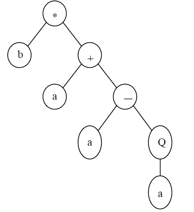
A K-expression can be mapped into an expression tree (ET) following a first-order procedure. A branch of the ET stops growing when the last node in this branch is a terminal. For example, the ET shown above corresponds to chromosome (2). In this case, the open reading frames end at position 7, whereas the gene ends at position 30.
Chromosomes in GEP are usually composed of more than one gene of equal length. For each problem or run, the number of genes, as well as the length of the head, is chosen. Each gene codes for a sub-ET and the sub-ETs can be linked by pre-defined rules forming a more complex multi-subunit ET.
Selection method and genetic operators: References [3] suggests there is no difference between different selection methods. It is strongly advised to use a simple elitism in any GEP implementation. The elitism means copying the best (or few best) individual to the offspring population without modifying them. GEP uses the well-known roulette-wheel method for selecting individuals.
In GEP, individuals were selected according to fitness by roulette wheel sampling coupled with the cloning of the best individual. The fitter the individual is, the higher the probability of leaving more offspring. Thus, during replication the genomes of the selected individuals are copied as many times as the outcome of the roulette. The roulette is spun as many times as there are individuals in the population, always maintaining the same population size.
GEP uses simple elitism of the best individual of a generation, preserving it for the next one. Replication is an operation that aims to preserve several good individuals of the current generation for the next one. In fact, this is a do-nothing probabilistic operation that takes place during selection (using the roulette-wheel method), and replicated individuals will be subjected to the action of the genetic operators. The mutation operator aims to introduce random modifications into a given chromosome. A particularity of this operator is that some integrity rules must be obeyed so as to avoid syntactically invalid individuals. In the head of a gene, both terminals and functions are permitted (except for the first position, where only functions are allowed). However, in the tail of a gene only terminal is allowed.
Mutation, Inversion, Transposition and Recombination
Mutation: Mutations can occur anywhere in the chromosome. Simple mutation just replaces symbols in genes with replacement symbols. However, the structural organization of chromosomes must remain intact. Symbols in the heads of genes can be replaced by functions or terminals (variables and constants). Symbols in the tail sections can be replaced only by terminals. Randomly change symbols in a chromosome. Symbols in the tail of a gene may not operate on any arguments. Typically two-point mutation per chromosome is used. It is worth noticing that in GEP there are no constraints neither in the kind of mutation nor the number of mutations in a chromosome: in all cases the newly created individuals are syntactically correct programs.
Inversion: Inversion reverses the order of symbols in a section of a gene. A portion of a chromosome is chosen to be inserted in the head of a gene. The tail of the gene is unchanged. Thus symbols are removed from the end of the head to make room for the inserted string. Typically a probability of 0.1 of insertion is used.
Transposition: Transposition selects a group of symbols and moves the symbols to a different position within the same gene. Gene transposition moves entire genes around in the chromosome. One gene in a chromosome is randomly chosen to be the first gene. All other genes in the chromosome are shifted downwards in the chromosome to make place for the first gene.
An IS element is a variable-size sequence of elements extracted from a random starting point within the genome (even if the genome was composed of several chromosomes). Another position within the genome is chosen as the insertion point.
This target site must be within the head part of a gene and cannot be the first element (gene root). The IS element is sequentially inserted in the target site, shifting all elements from this point onwards and a sequence with the same number of elements is deleted from the end of the head, so that the structural organization is maintained. This operator simulates the transposition found in the evolution of biological genomes. RIS is similar to the IS transposition, except that the insertion sequence must have a function as the first element and the target point must be also the first element of a gene (root).
The transposable elements of GEP are fragments of the genome that can be activated and jump to another place in the chromosome: (1) Short fragments with a function or terminal in the first position that transpose to the head of genes, except to the root (insertion sequence elements or IS elements); (2) Short fragments with a function in the first position that transpose to the root of genes (root IS elements or RIS elements); (3) Entire genes that transpose to the beginning of chromosomes.
Recombination: During recombination, two chromosomes are randomly selected, and genetic material is exchanged between them to produce two new chromosomes.
The cross over operation this can be one point (the chromosomes are split in two and corresponding sections are swapped), two point (chromosomes are split in three and the middle portion is swapped) or gene (one entire gene is swapped between chromosomes) recombination. Typically the sum of the probabilities of recombination is 0.7.
In GEP there are three kinds of recombination: one-point, twopoint, and gene recombination. (1) One-point: During one-point recombination, the chromosomes crossover a randomly chosen point to form two daughter chromosomes; (2) Two-point: In twopoint recombination the chromosomes are paired and the two points of recombination are randomly chosen. The material between the recombination points is afterwards exchanged between the two chromosomes, forming two new daughter chromosomes; (3) Gene recombination: recombines entire genes. This operator randomly chooses genes in the same position in two parent chromosomes to form two new off springs. In gene recombination an entire gene is exchanged during crossover. The exchanged genes are randomly chosen and occupy the same position in the parent chromosomes. It is worth noting that this operator is unable to create new genes: the individuals created are different arrangements of existing genes.
Fitness function: A fitness function is the most important part of any EA application. Fitness function given with above equations allows for fulfilling all of the set conditions. In GEP, fitness is based on how well an individual model the data. If the target variable has continuous values, the fitness can be based on the difference between predicted values and actual values. Evolution stops when the fitness of the best individual in the population reaches some limit that is specified for the analysis or when a specified number of generations have been created or a maximum execution time limit is reached.
All of the fitness functions produce fitness scores in the range 0.0 to 1.0 with 1.0 being ideal fitness – that is, the individual exactly fits the data. If a function is unviable – for example, it takes the square root of a negative number or divides by zero – then its fitness score is 0.0.
GEP evolution process: The GEP evolution begins with the random generation of linear fixed-length chromosomes for individuals of the initial population. The chromosomes are translated into ETs and subsequently into mathematical expressions, and the fitness of each individual is evaluated based on a pre-defined fitness function. The individuals are then selected by fitness to reproduce with modification. The individuals of this new generation are, in their run, subject to the same developmental process. The selection and reproduction is accomplished by roulette-wheel sampling with elitism, which guarantees the survival and cloning of the best individual to the next generation. Variation in the population is introduced by applying one or more genetic operators to selected chromosomes, including crossover, mutation and insertion.
Models
GEP model: The GEP program was coded by the combination of MATLAB and VC++. The MATLAB software has the advantage of computing matrix conveniently and programming efficiently, but its operating efficiency is relatively low. So VC++ was combined for its powerful function and the characteristics of higher operating efficiency with MATLAB. In this paper, MATLAB engine was used to achieve the combination with VC++ programming. There are two steps: (1) Add MATLAB engine library header files and library functions of the path. (2) Add libmx.lib libeng.lib libmex.lib to complete the import of the corresponding MATLAB engine static link library.
From the data in Table 1, GEP method was used that 6 topological index as input, output for its retention index. During the run, parameter values were needed to adjust constantly in order to achieve the optimal results. The set of optimal parameter values were listed in Table 2 and the predicting results of test set on OV-1 and SE-54 were listed in Figures 1 and 2. It can be seen from the figures that the predictive values of gas chromatography retention index of oxygen-organic compounds were in good agreement with the experimental data.
| Parameters | Values |
|---|---|
| Generation | 2000 |
| Population Size | 100 |
| Function Set | “+” “-“ “*” “/” “sin” “cos” “sqrt” “exp” “ln” |
| Head Size | 8 |
| Number Of Genes | 3 |
| Linking Function | + |
| Mutation Rate | 0.044 |
| 1-Point recombination rate | 0.3 |
| Gene recombination | 0.3 |
| Gene | 0.1 |
| IS transposition rate | 0.1 |
| RIS transposition rate | 0.1 |
| Gene transposition rate | 0.1 |
| Selection range | 100 |
Table 2: Parameters of GEP models.

Figure 1: Plot of the predicted RI against the experimental values on OV-1 column for test set based on GEP.

Figure 2: Plot of the predicted RI against the experimental values on SE-54 column for test set based on GEP.
ANN model: Non-linear statistical treatment of QSRR data is expected to provide models with better predictive quality as compared with related MLR models. In this perspective, functioning and applications of ANN have been adequately described elsewhere [7-10]. Extensive use of ANN, which has inherent ability to incorporate nonlinear and cross-product terms into the model and does not require prior knowledge of the mathematical function as well, largely rests on its flexibility and less sensitivity to collinearity among variables. The theory behind ANN and their use in chromatography have been reported elsewhere [11-13].
Multi-layer feed forward networks, with good self-learing ability and adaptability is widely used in the field of QSRR modeling [14]. Commonly, they consist of three layers: one input layer formed by a number of neurons that equal to the number of descriptors, one out neuron (providing the model response) and a number of hidden neurons fully connected to both input and out neurons. Among the available learning algorithms, back-propagation of errors is one of the most widely used [8,15].
Usually, there are four steps involved in ANN modeling: (1) assembling the training data of input (independent variables) and output (dependent variables), (2) deciding the network architecture, (3) training the network, and (4) simulating the network response to new inputs. The training process is simply an optimization process which aims at finding the set of weight and biases associated with each layer that will minimize the error objective function related to the deviations of the network predictions from the true response output data of the training set.
Before data set was used for the training of ANN, it was normalized separately. Its minimum value was set to zero and maximum to one. The proper number of nodes in the hidden layer was determined by training the network with different number of nodes in the hidden layer. The root-mean-square error (RMSE) value measures how good the outputs are in comparison with the target values. In this paper, following a troubleshooting study to investigate the effects of the number of hidden layers and the number of neurons involved in these hidden layers, a 2-3-1 network, with tansig-logsig transfer functions, was found to be the most optimum in terms of the root mean squared errors (RMSE) obtained.
ANN with basic back-propagation of errors learning algorithm was used in this study to predict oxygen-containing retention index. A three-layer network with a sigmoid transfer function was designed for ANN. The ANN program was coded in MATLAB 7 for windows [15].
The MLR: For regression analysis, data set was randomly divided into two groups: training and test sets. The training set, composed of 74 molecules, was used for the model generation. The test set, composed of 17 molecules, was used to evaluate the generated model. The program used for MLR analysis was compiled in Statistical Product and Service Solutions (SPSS version 19.0 IBM) software. In MLR analysis, in order to minimize the information overlap in descriptors and to reduce the number of descriptors required in regression equation, the concept of non-redundant descriptors was used in this study. The best equation was selected on the basis of the highest multiple correlation coefficients (R) and the lowest root mean squared error (RMS). The linear equation between these descriptors and the retention parameters of fluid catalytic cracking (FCC) gasoline was:
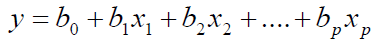 (1)
(1)
Where b0 is the intercept and bj is the regression coefficient for descriptor j. The statistical results obtained by using the two molecular descriptors based on MLR are listed in Table 3 and plotted against the experimental values in Figures 3 and 4.
| Descriptors | OV-1 coefficient | Std. Error | SE-54 coefficient | Std. Error | OV-1 test values | SE-54 test value |
|---|---|---|---|---|---|---|
| Constant | 1951.898 | 450.621 | 2028.14 | 345.24 | 4.332 | 5.875 |
| OEI | 48.089 | 4.351 | 50.562 | 3.333 | 11.053 | 15.169 |
| SX1CH | -43.038 | 151.408 | 3.36 | 116 | -0.284 | 0.029 |
| N2/3 | 3.331 | 51.507 | 26.672 | 39.462 | 0.065 | 0.676 |
| χeq ×PEI | -459.326 | 162.605 | -504.236 | 124.579 | -2.825 | -4.048 |
| χeq | -173.948 | 12.183 | -159.685 | 9.334 | -14.278 | -17.108 |
| MPEIm×IMPEIm | 5.589 | 1.039 | 5.694 | 0.796 | 5.382 | 7.156 |
Table 3: Model parameters value and coefficients for MLR model.

Figure 3: Plot of the predicted RI against the experimental values on OV-1 column for test set based on MLR.

Figure 4: Plot of the predicted RI against the experimental values on SE-54 column for test set based on MLR.
It is common to consider four statistical parameters for regression equation. These parameters are the number of descriptors, correlation coefficient (R) for training and test sets, root mean squared error (RMS) for training and test sets, and F statistic. A reliable MLR model is one that has high R and F values, low RMS and least number of descriptors. In addition to these, the model should have a high predictive ability. Consequently, among different models, the best model was chosen, whose specifications are presented in Table 3. Here the corresponding descriptors used in MLR were applied as inputs for ANN in order to compare the performance of the two models.
The main aim of the present work was developing a QSRR model to predict the retention parameter (RI) of oxygen-containing compounds appeared in Table 1. A linear model of MLR was developed, whose specifications are given in Table 3. All statistic tests were performed at a significance level of 5%. MLR model performance was measured by three metrics: (1) R, which gives the fraction explained variance for the analyzed set, was used to measure the model’s fit performance. (2) Root Mean Squared error (RMS), which can give the bias in the prediction, was used to evaluate the model’s predictive precision: the lower the RMS, the better the prediction precision. It can be calculated as below:
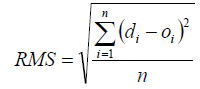 (3)
(3)
where di is the target value, oi is the experimental value and n is the number of compounds in analyzed set. (3) The variance ratio of calculated and observed activities F.
After the linear model was gained, non-linear characteristics of the retention parameter were also performed using ANN. Here a feedforward neural network with basic error back-propagation algorithm was constructed to model the nonlinear QSRR models. Therefore, a 2-3-1 BP-ANN, with tansig-logsig transfer functions, was developed. Figure 5 demonstrates the plot of the ANN predicted versus the experimental values of the RI for the data set. A correlation coefficient of this plot indicates the reliability of the model. As can been seen in Table 4, the correlation coefficient R on OV-1 and SE-54 for the ANN models are larger than that of MLR models respectively, which indicates that the ANN models are slightly improved to MLR models. The residuals of calculated values of RI by ANN are plotted against the experimental values in Figure 6. The propagation of the residuals on both sides of zero line indicates that no symmetric error exists in the development of ANN model.

Figure 5: Plot of the predicted RI against the experimental values on OV-1 column for test set based on ANN.

Figure 6: Plot of the predicted RI against the experimental values on SE-54 column for test set based on ANN.
| OV-1 | Test sets | SE-54 | Test sets |
|---|---|---|---|
| Method | R | Method | R |
| MLR | 0.9911 | MLR | 0.9917 |
| ANN | 0.9891 | ANN | 0.9892 |
| GEP | 0.9909 | GEP | 0.9955 |
Table 4: Result of correlation coefficient (R) with MLR, ANN and GEP for the test set.
Correspondence author is grateful to the financial support from National Natural Science Foundation of China, Lanzhou University of China and Liaoning Province Education Department of China, which made this work possible.