Journal of Thermodynamics & Catalysis
Open Access

Performance Analysis of a Fin in Steady State

Mindi Ramakrishna^1*, N Chitti Babu², Boddu Manisha¹ and G Durga Venkata Nagesh^{1 *}Correspondence: Mindi Ramakrishna, Department of Chemical Engineering, Rajiv Gandhi University of Knowledge Technologies, Nuzvid, Andhra Pradesh, India, Email:

Author info »

Introduction

The effect of removal of waste heat or excess heat to another material or medium by using any external means such as fans, blowers or extended fin surfaces has been essential to smoothly run the chemical engineering heat transfer applications. In order to maintain this condition with unduly increasing the weight of device, the material used and hence cost of applications, extended surfaces are often used. As the rate of convective heat transfer depend on area of heat transfer surface, one can enhance surfaces called ‘fins’. The literature denoted to numerical analysis of fins. In the present study specifically focused on the aspect of “performance analysis of a fin in steady-state” [1-5].

The study of heat transfer and fluid dynamics has a pivotal role in various engineering domains, especially in the design and optimization of heat exchangers, aerospace structures, and cooling systems. One crucial element in these systems is the fin, a protruding surface intended to enhance heat transfer by increasing surface area. Understanding the performance of fins in steady-state conditions is fundamental to evaluating their efficiency in dissipating heat or enhancing convection.

This performance analysis aims to delve into the intricate details of fins operating under steady-state conditions. By examining how fins interact with fluid flow and temperature gradients, this investigation seeks to provide comprehensive insights into the factors influencing their effectiveness in heat transfer applications. Through meticulous analysis and empirical data, this study endeavors to elucidate the thermal characteristics, efficiency, and limitations of fins operating in steady-state conditions.

The exploration of fin performance in steady-state conditions encompasses various parameters, including fin geometry, material properties, fluid properties, and environmental conditions. By systematically evaluating these factors, this analysis endeavors to offer a deeper understanding of the thermal behavior of fins and their impact on heat dissipation or transfer rates.

Ultimately, this research intends to contribute to the advancement of engineering practices by providing valuable insights into optimizing fin design and configuration for enhanced heat transfer performance in steady-state conditions.

Methodology

Shooting method

The shooting method uses the methods used in solving initial value problems. This is done by assuming initial values that would have been given if the ordinary differential equation were a initial value problem. The boundary value obtained is compared with the actual boundary value. Using trial and error or some scientific approach, one tries to get as close to the boundary value as possible.

Developing model equation

Consider a fin which approximately in the shape of parabola (Just approximated) . The temperature distribution is taken as function of distance from it’s base i.e., T (x). Radius at each ‘x’ is varied as r (x).

Taken expressions are:

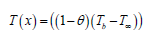
Where

h=convective heat transfer coefficient.

k=heat conduction coefficient.

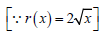(Since, Axis starts from right to left side. (for x>0))

Here A (x) = Cross sectional area as function of x.

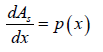
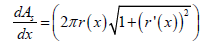
The expression for perimeter of cross section at taken ‘x’ distance from base is given as:

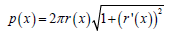
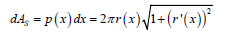
Hence, if a differential region with in the fin is considered, then differential surface area=dAs

Hence,

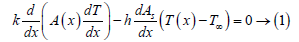
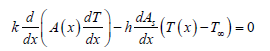
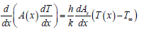
Total energy balance equation

{Rate of energy in due to conduction} - {Rate of energy out due to conduction and convection}=0

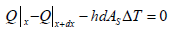
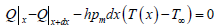
(By using tayler’s series expanision and fourier’s law of conduction)

So, perimeter

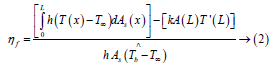
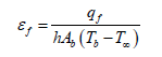
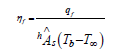
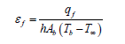
From the formula of “Efficiency”:

Q_max can be found when the whole fin surface is maintained at base temperature (i.e. maximum temperature gradient occurs).

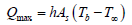
So,

Where,

T_b=Temperature at the base.

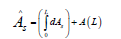
Hence,

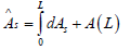
Here heat transfer surface area (i.e. sides surface area+bottom surface area)

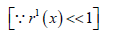
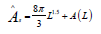
Hence,

(:- since it is non-vanishing thickness)

Therefore,

Effectiveness of fin

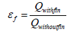
If there is no fin, then total heat transfer is only from base [6,7].

Where

A_b=Area of base

T_b=Temperature at base

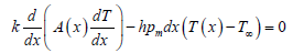
Numerical solution for (equation 1) to find temperature profile as a function of distance (x) from base and also as a function of radius (r(x)).

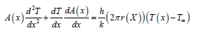
Consider equation 1:

Then,

Hence,

From UV rule of integration

From above results, since it is a 2^nd order non linear equation, we are approximating the solution

using Shooting Method.

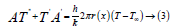
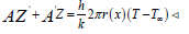
Let’s say

T’=Z

T”=Z

Substitute above two considered variable in equation (3)

From (3)

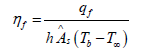
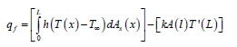
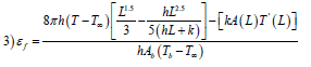
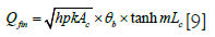
To find Efficiency And Effectiveness, We need expression for ‘q_f’ So,

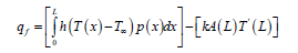
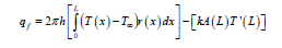
‘h’ is taken as not function of x (in assumptions)

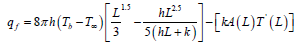
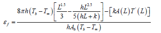
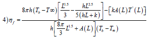
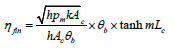
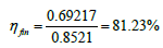
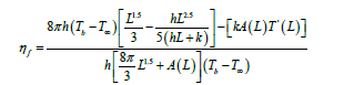
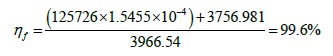
Hence, Efficiency:

Hence,

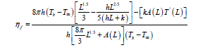
As ‘L’ varies, ‘η_f’ get varied.

Where L=Total length of fin from its base.

Similarly:

Effectiveness:

To find є_f and η_f, we should just substitute the value of ‘L’ (i.e. length of fin). Since all other parameters are kept constant.

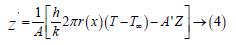
Now, to obtain plot to observe the variation of temperature in the fin, Take equation (3)

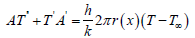
Here,

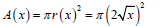
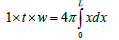
A(x) = 4πx

A^'(x) = 4x

Hence from taken equation (4)

By using these equations, we can solve by MATLAB and obtain the solutions for finding temperature profiles as a function of ‘x’.

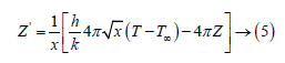
Final equations are:

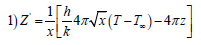
2)T ' = Z

Performance analysis of parabolic FIN

Problem statement: One-dimensional and steady-state heat transfer in an extended fin of shape that approximately resembles parabola with one end attached to a surface at base temperature of 350°C. The fin is made of aluminium whose thermal conductivity is k = 235(w/ m°k), the heat transfer cofficient with respect to surrounding fluid is h =154(w/ w/ m^∧ 2° k) which is maintained at a temperature of T_∞=25°C. The length of parabola is ‘L’. Area of cross section varies as 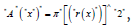and temperature variation is denoted by T(x), where ‘x’ indicates the direction of fin length from the surface. The Figure 1 is shown below. The fin is studied under the case where convective heat transfer occurs at the tip. The solution should utilize the numerical approach. To determine the plot for temperature variable along the fin length and compare it with regular rectangular fin’s temperature profile under the same conditions with length=0.05 m, thickness=0.005 m, width=1 m. In addition to it, compare the efficiencies in both cases by considering both the fins are maintained at same volume.

Figure 1: Schematic Diagram of Parabolic Fin. Note: D: Heat transfer; The conduction coefficient (k) and the convective heat transfer coefficient h are constant; The temperature T_b of the fin base is constant; The temperature T_∞ of the surrounding fluid is constant.

Assumptions

1. Heat transfer is 1-D.

2. Heat transfer is steady-state.

3. Radiative heat transfer is negligible.

4. The conduction coefficient k and the convective heat transfer coefficient h are constant.

5. The temperature T_b of the fin base is constant.

6. The thermal contact resistance between the surface and fin is negligible.

7. The temperature T_∞ of the surrounding fluid is constant. We make the following additional assumptions.

8. The fin is a body of revolution.

9. The cross-sectional area decreases in the direction away from the surface.

From the give data

h = 154 (w/ m².k)

k = 235 (w/ m.k)

T_b = 350°c

T_∞ = 25°c

Substituting the data in the expression of Z’ and Z (i.e. eqn 1 and eqn 2). As we know for the case of rectangular fin with convective heat transfer occurs at the fin tip whose fin length is finite, the temperature variation along the length of fin is,

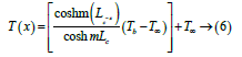
From given data, use equations (1), (2) and (6), and plot the temperature profiles in both the cases as function of length of fin, using MATLAB . Simulations are done using shooting method [8].

Comparison between rectangular and approximated parabolic fins by taking equal volume of fins

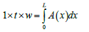
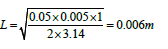
Volume of rectangular fin=length × thickness × width=1×t ×w

Volume of approximated parabolic fin=

Compare the volumes to analyze the case,

From data,

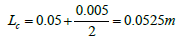
Rectangular face with convective heat flux at the tip:

Where

l=length of fin

t=Thickness of the fin.

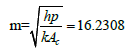
From data,

So , here h=heat transfer coefficient (w/m².k)

p=Perimeter of fin (2×(w+t))

k=Thermal conductivity

Ac=Cross sectional area (t×w)

Comparison of effectiveness of both the fins

In rectangular fin:

[10]

In approximated parabolic shaped fin:

L = 0.006m

A(L) = 4πL = 0.07536m²

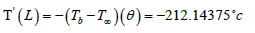
From data,

Results and Discussion

The plot signifies the variation of temperature along length of fin is exponentially decreasing in both the cases. For the same length of fin from origin, the temperature drop in approximately parabolic shaped fin is higher than that in rectangular fin. This indicates that, since all other parameters are kept same, in approximated parabolic shaped fin-The profile is more optimized than that of regular rectangular fin’s profile. This indicate rate of heat loss is higher in considered case of fin rather than that in rectangular fin.

The steady state and one-dimensional temperature distribution along the length of approximated parabolic shaped fin is studied and profile of regular rectangular fin under same conditions is drawn in Figure 2. Efficiency of considered fin is determined and found that this efficiency is higher than the rectangular fin’s efficiency. Hence optimal study of a fin under steady state is analyzed.

Figure 2: Temperature distribution in parabolic and rectangular fins.

Conclusion

The project involves the study of temperature distribution along length of fin for a approximated parabolic fin. The non-linear differential equations are simulated using shooting method in MATLAB. The efficiency of the fin is found to be more than that of rectangular fin’s efficiency for the same specifications and of equal volume. Hence, this can enhance rate of heat transfer and then enhances efficiency. Finally, it can minimize expenses.

References

1. Belinskiy BP, Hiestand JW, Weerasena L. Optimal design of a fin in steady-state. Applied Mathematical Modelling. Electron J Differ Equ. 2020 ;77:1188-2200.[Crossref]

   [Google Scholar]

2. Hanin L. A new optimum pin fin beyond the “length-of-arc” assumption. Heat transfer engineering. Heat Transf Eng. 2008;29(7):608-614.

   [Crossref][Google Scholar]

3. Singla RK, Das R. A differential evolution algorithm for maximizing heat dissipation in stepped fins. Neural Computing and Applications. Neural Comput &Appl. 2018;30(10):3081-3093.

   [Crossref][Google Scholar][PubMed]

4. Yu LT. Application of Taylor transformation to optimize rectangular fins with variable thermal parameters. Appl Math Model.1998;22(1-2):11-21.

   [Crossref][Google Scholar]

5. Bergman TL. Fundamentals of heat and mass transfer. seventhed John Wiley & Sons, NewYork. 2011.

   [Google Scholar]

6. Belinskiy BP, McCarthy CM, Walters TJ. Optimal design of turbines with an attached mass. ESAIM: Control, Optimisation and Calculus of Variations. Eur Ser Appl & Industr Math .2003:217-230. [Google Scholar]
7. Belinskiy BP, Hiestand JW, Matthews JV. Piecewise uniform optimal design of a bar with an attached mass. Electron J Differ Equ. 2015(206):17.

   [Google Scholar]

8. Barman D, Goswami D, Kundu B. An optimum longitudinal wet fin without the “length-of-arc” assumption. HVAC & R Res. 2013;19(4):444-456. [Crossref]

   [Google Scholar]

9. Hanin L, Campo A. A new minimum volume straight cooling fin taking into account the “length of arc”. Int J Heat Mass Transf. 2003;46(26):5145-5152.

   [Crossref][Google Scholar]

10. Belinskiy BP, Hiestand JW, McCarthy ML. Optimal design of a bar with an attached mass for maximizing the heat transfer. Electron J Differ Equ. 2012;13:181.

    [Crossref][Google Scholar]