Angiology: Open Access
Open Access

Enhancing Early Detection of Cardiovascular Diseases through Deep Learning-Based ECG Signal Classification

Author info »

Introduction

CVD is the leading cause of death, based on statistics from the American health monitoring organisation and the Centres for Disease Control and Prevention (CDC) [1]. The CDC reports that heart disease affects a staggering 74% of the population annually. The prevention of CVDs hinges on early and accurate diagnosis [2]. The realm of modern medical science has unveiled potent solutions for addressing heart-related issues, leveraging advanced information technology techniques. Among the most common methods for detecting heart disease are angiography, ECG, and blood tests [3]. The ECG, which is frequently used as a diagnostic aid for screening CVD, includes recording visual signals by inserting electrodes into the skin of the person to track voltage changes. ECG serves to detect potential cardiac abnormalities, particularly in the ST segments [4]. Typically, it identifies changes such as ST-segment elevation or depression, T wave alterations, or the appearance of new Q waves-these deviations signify symptoms of cardiac disease [5]. Traditionally, cardiologists manually interpret ECG results based on diagnostic criteria and their experience. However, manual interpretation is time-intensive and demands expertise [6]. Misinterpreted ECG results can lead to incorrect clinical decisions, posing risks to human life and well-being. Given the rapid improvement of ECG technology and the scarcity of cardiologists, reliable and automated identification of ECG signals has emerged as an attractive study topic for many academics.

Several efforts were made over the last decade to discover acute ECG patterns by employing 12-lead ECG data, especially using freely accessible open-source ECG databases [7,8]. While these methods anticipate results with excellent accuracy based on one-dimensional ECG rhythms, they have yet to acquire broad acceptance in healthcare organizations. One of the key challenges in applying Machine Learning (ML) to ECG analysis is feature extraction [9]. Current classification systems extract medical features through signal-processing techniques. These systems integrate the extracted features and compare them with features derived from various heart diseases. However, due to noise interference, some features are challenging to extract. Moreover, different CVDs exhibit distinct ECG signal features, making it impractical to design a system that can capture all the necessary features. Consequently, these diagnostic systems suffer from poor scalability and reduced accuracy. Recently, DL techniques have emerged as a positive solution for ECG interpretation [10]. In this work, we employ DL models to automatically extract features from the raw ECG signals.

Literature survey

In this section, we will delve into a thorough examination of the latest developments in the field of CVD detection through the use of ECG signals. Recent researchers in this subject have opened the way for spectacular achievements and creative approaches that offer suggest enhancing the early identification, evaluation, and tracking of CVD illnesses. In the study, DL approaches are used to identify four significant CVDs from ECG signals [11]. The study looks at transfer learning using pre-trained Deep Neural Networks (DNN) like SqueezeNet and AlexNet. Furthermore, the authors suggest a unique CNN framework designed specifically for CVD prediction. Particularly, these DL models can also be used to extract features from standard ML algorithms such as K-Nearest Neighbors (KNN), Support Vector Machine (SVM), Random Forest (RF), Decision Tree (DT), and Naive Bayes (NB). The findings show that the suggested CNN model achieves outstanding performance. When employed for feature extraction, it surpasses existing algorithms, achieving the greatest score with the NB approach. The study introduces a set of ML models aimed at solving the challenge of ECG-based CVD detection [12]. Mechanisms for data collection and training techniques for multiple algorithms are accounted for in the models. The authors integrate the heart dataset with additional classification models to validate the success of their technique. The suggested method outperforms other current methods with about 96% accuracy and provides a comprehensive analysis across several variables. The study emphasizes the potential value of new data from various medical institutions in improving the creation of artificial neural network architectures and so contributing to the field of DL. The fundamental goal of this suggested model is to improve the accuracy of ECG-based CVD categorization by using a hybrid feature engineering technique [13]. The model is made up of three major parts: Pre-processing, integrated feature extraction, and categorization. The goal of the pre-processing step is to remove baseline and powerline interference while keeping heartbeat information. A hybrid technique is developed for effectively recognizing the data, combining traditional ECG rhythm-extracting techniques with CNN-based features. The generated hybrid feature vector is subsequently fed into the Long Term Short Memory (LSTM) model. The simulation findings show that the suggested approach minimizes diagnostic mistakes and the time necessary to conduct a diagnosis when compared to existing techniques.

The research focuses on the creation of a bimodal CNN developed on gray images and ECG scalograms for CVD diagnosis [14]. The study makes use of a 12-lead ECG data, including 10,588 ECG records labelled by a professional physician. One- dimensional ECG data are converted to scalograms and two- dimensional grayscale images, which are used as dual input images for the suggested CNN framework. The model, which is made up of two similar Inception-v3 backbone designs, performs admirably, with high positive metrics. The bimodal CNN surpasses conventional categorization techniques trained solely on gray images or scalograms, providing an important instrument for CVD diagnosis. The paper provides a system for predicting, categorizing, and improving the diagnostic efficacy of CVDs using multiple ML algorithms [15]. To identify CVD risk factors, various ML strategies are used. For dealing with continuous and categorical variables, mixed-data transformation and categorization algorithms are used. Employing a real CVD data sample acquired from a hospital, the research compares hybrid models to current ML approaches in depth. The results show that the suggested methodology outperforms well-known statistical and ML methodologies, with ANFIS attaining the most accurate predictions. The work describes a DL-based system that uses CNNs to classify ECG signals from the MIT- BIH Arrhythmia dataset [16]. A 1-D convolutional deep ResNet model is used in the suggested technique to extract features from the heartbeats. To overcome class imbalance throughout training, the Synthetic Minority Oversampling Method (SMOTE) is used, effectively identifying 5 heartbeat patterns in the test data sample. The effectiveness of the classification model is evaluated using ten-fold cross-validation, displaying high metrics scores. The suggested ResNet (Residual Neural Network) model outperforms other 1-D CNNs in ECG signal categorization, demonstrating its usefulness.

The research focuses on detecting both regular and abnormal ECG signals [17]. Since there are many different kinds of noise present in ECG data, this study suggests a record-filtering strategy to get rid of those. Furthermore, a feature fusion method is created for obtaining both global and local characteristics from various ECG leads, resulting in the construction of an accurate depiction of the ECG record. RF, Multi-Layer Perceptron (MLP), and modified ResNet are among the classification baselines used. Ensemble approaches are also investigated, which combine RF with ResNet and MLP. When compared to many state-of-the- art approaches on the same database, the hybrid model, which uses RF and modified ResNet, provides the most effective outcomes for classification. The study focuses on classifying various CVDs using bio-inspired algorithms with and without hyper parameter optimization [18]. ECG signals are subjected to dimension reduction methods such as linearity preserving projection, principal component analysis, variational bayesian matrix factorization, and Kernel-linear discriminant analysis. Whale optimisation, particle swarm, grey wolf, fish swarm, KNN, SVM with RBF kernel, and NB are used to classify ECG signals after reducing their dimensionality. The paper presents accurate findings for classification algorithms with and without hyperparameter tuning. Particularly, hyperparameter optimization using the Adam and Randomised Adam (R-Adam) techniques improves the efficiency of classifiers significantly, with the Grey Wolf-R-Adam classifier obtaining exceptional overall accuracy in categorizing CVD. The paper provides a DL and fuzzy clustering- based technique (Fuzz-ClustNet) for detecting arrhythmias in ECG signals [19]. The study starts with denoising ECG readings to eliminate defects. Data augmentation is conducted to solve the class imbalance. For extracting characteristics from augmented images, a CNN feature extractor is used, which is then fed to a Fuzz-ClustNet method for ECG signal categorization. Multiple simulations are run on benchmark datasets, and the results are analysed using a number of performance measures. The finding indicates the efficiency of the suggested approach in detecting CVD from ECG signals when compared with existing approaches.

Materials and Methods

This section comprehensively discusses the methodologies employed for CVD detection using a DL approach, presenting a step-by-step breakdown of the entire process.

Data

In this study, the PTB-XL ECG database was utilized [20]. It represents a clinical ECG dataset of an unprecedented scale, modified to assess the performance of ML algorithms. This extensive dataset comprises 21,837 clinical 12-lead ECG recordings from 18,885 individuals. These recordings are 10 seconds in duration and are sampled at both 500 and 100 Hz, with 16-bit resolution. Figure 1 provides illustrative examples of various ECG rhythms, which align with the data detailed in Table 1 and were employed in the research. These examples encompass a range of ECG signals, including normal patterns, conduction disturbances, ST/T changes, MIs, and hypertrophy. Figure 2 illustrates the sample ECG signal from each class.

Furthermore, it's worth noting that the PTB-XL database maintains gender balance, consisting of data from both male (52%) and female (48%) patients, spanning an age range of 2 to 95 years (with a median age of 62). This dataset is supplemented with additional patient details like age, gender, height, and weight. The authors of the dataset have meticulously categorized each ECG into 23 diagnostic subclasses within five diagnostic classes, or alternatively, into non-diagnostic classes. Each class is associated with a corresponding probability. These classes are identified using the standard codes SCP_ECG.

Table 1: PTB-XL database.

Figure 1: ECG data distribution in percentage. Note: Normal;

Figure 2: Sample ECG signals of CVD.

Data processing

processing The data sourced from the PTB-XL database underwent a series of pre-processing steps and was subsequently partitioned into training, validation, and test subsets. During the pre-processing stage, the data was subjected to filtering and normalization to ensure its suitability for examination using the DL model [21]. The presence of noise in ECG signals can significantly hinder the identification of representative ECG patterns and may lead to erroneous interpretations [22,23]. Within ECG signals, two prominent types of noise exist, including electromyogram noise and additive white Gaussian noise, both of which are characterized by high frequencies. Low pass filtering is employed for denoising ECG signals to mitigate the impact of noise. Subsequently, in the pre-processing workflow, the normalization step was carried out to address negative signal values. This normalization is important to ensure that both normal and abnormal signals do not contain negative values. In essence, the normalization process aims to simplify the raw signal extracted from the PTB-XL Database before developing a system capable of distinguishing between normal and abnormal ECG signals. The normalization formula for obtaining Ns involves finding the minimum value from the signal v and subtracting it from v_n, representing the value of the successive signal with the minimum value it shown in equation 1.

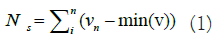
N_s serves as a processed signal that facilitates the detection of the positions and values of P, Q, R, S, and T signals in both normal and abnormal ECG signals. Finally, the dataset was partitioned into three subsets: Train, validate, and test, with percentages of 80%, 10%, and 10%. The 80% of the sample was utilized to train the DL network, the 10% sample aided in model validation, and the last 10% was instrumental in evaluating the network's performance.

Deep learning

The architecture and working of the DL network including ResNet-50, Inception-V3, and CNN-VAE are discussed below.

ResNet-50: The ResNet has garnered impressive results in various visual recognition competitions [24]. One of the key issues it addresses is the gradient disappearance problem, which is a significant reason for its adoption in this study [25]. ResNet is a development of VGG19 that introduces residual units via a short- circuit method, downsamples with convolution using a stride of 2, and replaces Fully Connected Layers (FCL) with global average Pooling Layer (PL). The ResNet model employs two basic types of residual components [26,27]. The shallow network is a construction block, while the deep network is the bottleneck block. There are two ways to enter information. The first is the identity mapping, it guarantees long-term memory retention. If enhancements are required, they are applied through direct mapping, denoted as f(x). Improved f(x) facilitates information flow between blocks, leading to enhanced model performance.

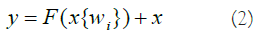
The residual structure's major purpose is to allow the NN to preserve its core identity mapping capabilities. This functionality guarantees that the training outcomes remain intact when networks are layered. Assuming that the NN's input and output parameters (x and h(x)), and the internal structure of H(x) are not explicitly described. ResNet allows the submodule to learn the residual f(x)=H(x)-x directly, resulting in the desired outcome F(x)+X. This prevents the efficiency and accuracy deterioration that might occur when there are too many Convolution Layers (CL). The result of the preceding layer is added to the result of this layer via the shortcut link, and then the sum is passed to the activation function. The shortcut connection of ResNet might be stated as (Equation 2).

For normal data, the correlation between the input data and the NN's outcome could be characterized as follows, taking into account the ReLU activation function and the double-layer weights (Equation 3).

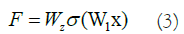
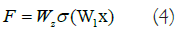
Typically, the ReLU activation function introduces nonlinearity and connects the weights W₁ and W₂ of the function and structure layers. To adjust the dimensions of the input and output data, a linear transformation WS is applied to x when creating a shortcut, as follows (Equation 4):

The ResNet-50 network framework was used in this research because of its broad use in image feature retrieval across multiple areas. The residual element of the ResNet-50 successfully handles the problem of network depth degradation. Furthermore, it addresses issues linked to shallow network layers' restricted potential for learning and inadequate feature extraction efficiency. Figure 3 depicts the ResNet -50 model's architecture, which consists of 50 layers organized into four major components. The initial component is made up of three smaller components, the subsequent component is made up of four smaller components, the third component is made up of 6 smaller components, and the final component is made up of 3 smaller components. Each tiny component has three convolutional cores. The 50-layer network framework is formed by a CL in the initial and a FCL in the last.

Figure 3: ResNet-50 architecture.

Inception-v3: The Inception model, introduced by Szegedy et al. during the 2016 Large-Scale ImageNet Visual Identification Challenge, was designed to address issues related to computational efficiency and parameter count in practical applications [28]. Inception-v3 takes input images sized at 299 × 299, which is 78% larger than VGGNet (244 × 244), yet it exhibits faster processing speed. This efficiency can be attributed to several factors: Inception-v3 has fewer parameters compared to AlexNet, with fewer than half (60,000,000) and less than one- fourth (140,000,000) of the parameters found in AlexNet [29] and VGGNet [30], respectively. Furthermore, the total amount of floating-point computations in the Inception-V3 model is around 5,000,000,000, which is considerably greater than in the Inception-v1 system (1,500,000,000). Because of these features, Inception-v3 is extremely practical and suited to be deployed in ordinary servers, allowing for immediate response.

Inception-v3 employs convolutional kernels of various sizes, allowing it to possess receptive fields covering different areas. To streamline the network design, it employs a modular system followed by feature fusion, enabling the integration of features from multiple scales. The network architecture comprises a series of CL and PL. Initially, CL-1 employs a 33-patch size and a stride of 2. Subsequently, CL-2 and CL-3 utilize a 33-patch size with a stride of 1. Following this, pool layer-1 adopts a 33 patch with a stride of 2. CL-4 employs a patch size of 33 and a stride of 1, while CL-5 uses a patch size of 33 and a stride of 2. CL-6 also utilizes a patch size of 33 with a stride of 1. These layers are followed by three inception blocks, five inception blocks, and two inception blocks. Finally, PL-2 employs a patch size of 8 × 8. The activation function employed for classification in this architecture is SoftMax. The model's configuration is depicted in Figure 4.

Figure 4: Inception-v3 Architecture. Note: pooling.

A Batch Normalisation (BN) layer was added in Inception-v3 as a regularizer between the auxiliary and the FCL. The BN network uses batch gradient descent to speed up training and enhance model convergence in DNNs. These are the expressions of the BN formulas in below equations from 5-10:

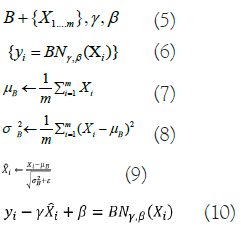
Where, X represents the minimum activation value within batch B, γ, and β indicate learning parameters, m represents the total activation values, σ_B² represents the standard deviation in each feature map dimension, μΒ represents one dimension’s average value, and ε is a constant. Convolution and pooling processes are performed in parallel with Inception-v3's use of an approach in which giant convolution kernels are separated into smaller ones. In addition, it provides smoothing-criterion-based labels for regularisation. Inception-v3 adds BN by normalizing the input at each layer, optimizing the learning process to overcome input-output distribution inequalities that cause issues for feature extraction in conventional DNN.

CNN-Variational Autoencoder (VAE): Convolutional Neural Network (CNN); a CNN is a type of NN featuring multiple layers, like CL and PL, as well as a FCL [31,32]. The standard CNN design aims to recognize image shapes while retaining partial invariance to their location within the image. In the CL, input images are convolved with 2-D filters, denoted as K. For instance, given a 2-D image I as input, the convolution operation is represented as follows in equation 11:

Subsequently, the feature maps resulting from the convolution operation are downsampled in the PL. The network learns the weights and filters (kernels) in the CL using backpropagation to minimize classification errors. In our dataset, we simultaneously use electrode location, time, and frequency data. Vertical activation locations are particularly important for classification performance, while horizontal activation locations are less significant. Therefore, in this experiment, the kernels applied are of the same height as the input image but have 1D filters horizontally. The network is trained using a total of T_F=30 filters. Input signals are convolved with these training kernels, and an output map in the CL is generated through the output function f in equation 12:

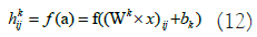
Here, x represents the input image, W^k and b^k indicates the weight matrix and bias value for k=1,2,...,T_F. The chosen output function f is the ReLU function in below equation 13:

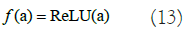
The CL’s output consists of T_F vectors of dimensions (Nt-2) × 1. The following max-PL uses zero padding, resulting in the output map being subsampled into T_F vectors of 1D. The layer that follows max-PL is an FCL with five neurons that indicate ECG categorization. To train the CNN parameters, the backpropagation technique is used, with error E calculated based on the difference in the desired and the network's output. The gradient descent approach is then used to minimize the error E by modifying the network parameters using the equations 14,15.

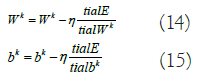
Here, η represents the learning rate, W^k signifies the weight matrix for kernel k, and b^k denotes the bias. The trained network will be utilized to categorize test samples.

Variational Autoencoder (VAE): The goal of an AutoEncoder (AE) NN is to have the output exactly match the input. The input is encoded in a hidden layer (h) that is part of the network's architecture. Where x is the input, the decoder function r=g(z) and the encoder function z=f(x) are the two main building blocks of the network. One method to get useful information out of an AE is to make z have fewer dimensions than x. Under completeness in an AE occurs when the dimension of the code is less than the input. In order for the AE to learn an incomplete representation, it must prioritize which elements of the training data are most important. The VAE is a directed model that requires just gradient-based approaches for training and relies on approximate inference learned from data [33-35].

First, it takes a random number z from the code distribution _pmodel(z) to create samples from the VAE model. A generator network g(z) capable of differentiation is then applied to the sample. The last step is to draw x at random from the distribution _pmodel(x;g(z))=_pmodel(x|z). The encoder q(z|x) is used to acquire z during training, while _pmodel(x|z) is considered as a decoder network. Maximizing the variational lower bound L(q) for the data point x is the main idea underpinning VAEs' training strategy:

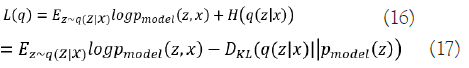
The first element in Equation (16) indicates the joint log- likelihood of hidden and visible elements. The entropy of the approximation posterior is the second element. Maximizing the entropy term stimulates a rise in the standard deviation of the noise when q is selected as a Gaussian distribution with noise introduced to a projected mean. More broadly, this entropy maximizes the variational posterior to attribute high probability to a range of z values from which x may have been formed, rather than a single point estimate. The first element in equation (17) is the reconstruction log-likelihood that appears in other AEs. The second element attempts to make q(z|x) a posterior distribution that is consistent with _pmodel(z). The network can deal with stochastic inputs, and stochastic gradient descent has trouble with stochastic nodes. The "reparameterization trick," by which the sample is moved to an input layer, solves the problem. By picking from the range ~ N(0,I), we can generate a sample from the distribution N(μ(x),θ(x)), from which we can calculate Pmodelz=μ(x)+θ^1/2(x) ϵ. Assume that q(z|x) has a mean and a covariance of μ(x) and θ(x), respectively. Therefore, the solution to Equation (17,18) is as follows:

The VAE has three layers: Input, AEs, and output. Unsupervised training is used for each AE layer in the deep network, with the output of the prior AE's hidden layer feeding into the input of the following AE. After this initial phase of training, the network's parameters are trained via the backpropagation method in a supervised fine-tuning phase.

Combined CNN-VAE: The data collected from an ECG is relatively weak and subject to interference [36]. Artifacts add difficulty by triggering irrelevant effects that damage the actual ECG patterns. The existence of artifacts, channel correlations, and the immense dimension all make developing an appropriate ECG classification system problematic. To address these issues, we offer a novel DL approach that includes a CNN accompanied by a VAE, as shown in Figure 5.

Figure 5: CNN-VAE architecture.

In this DL construction, we first use CNN to analyse input and train network parameters alongside the kernels. Following that, the result of CNN is employed as an input to VAE model. The VAE's input stage is made up of 700 neurons. The CNN-VAE model is used in this structure to represent the spectral, temporal, and spatial aspects of ECG, which improves classification accuracy.

The CNN-VAE used in testing has a computational complexity of O(N_h × N_t × N_F × N_FS)+O((N_t × N_F)² × N_L). The computational complexity of the CNN is shown by the first element, where N_h × Nt is the size of the input image, N_Fs is the number of convolution kernels, and N_F is the size of the kernel. The computational complexity of the VAE is represented by the second element, where NL is the number of total layers. Since the VAE network is fully connected, the complexity includes a squared term.

Results and Discussion

Here, we demonstrate the results and discuss the efficiency of three DL models for CVD detection with ECG data: ResNet-50, Inception-V3, and CNN-VAE. To evaluate the efficacy of the DL models during the training phase, graphical representations of both accuracy and loss were developed. The x-axis of these plots represents the iterations used to train the model. The performance of the models is visualised along the y-axis, which shows both loss and accuracy values.

Training phase

The accuracy plot for ResNet-50 in Figure 6 demonstrates a consistent increase in both training and validation accuracy as the number of training epochs progresses. Notably, there are significant improvements observed within the initial 15 epochs, followed by diminishing growth. By the end of training, the model attained a training accuracy of 88.67% and a validation accuracy of 89.73%. The minimal difference between these two accuracies indicates that the model generalizes effectively to unseen data. Similarly, the loss plots illustrated in Figure 7 showcase a continual decrease in both training and validation losses, resulting in values of 26.33% and 30.21%, respectively.

Figure 6: RESNET-50 accuracy performance on training phase.

Figure 7: RESNET-50 loss performance on training phase.

In Figure 8, the accuracy plot for Inception-v3 demonstrates an upward trend as the number of training epochs increases, with most substantial improvements occurring within the first 12 epochs. Overall, the model undergoes 50 epochs, achieving a training accuracy of approximately 93.11% and a validation accuracy of around 89.43%. As shown in Figure 9, the loss curves exhibit a decreasing pattern with epochs, concluding at a training loss of approximately 22.22% and a validation loss of approximately 29.18%. These results indicate the model's strong generalization capacity.

Figure 8: Inception-v3 accuracy performance on training phase.

Figure 9: Inception-v3 loss performance on training phase.

Figure 10 portrays the accuracy plot for CNN-VAE, showcasing a remarkable increase in recognition training accuracy, reaching around 90% by the 11^th epoch and eventually reaching a peak recognition training accuracy of 97.71% after 20 epochs. Similarly, the recognition validation accuracy increases steadily, reaching approximately 90% by the 22^nd epoch and achieving a maximum of 96.8% after 44 epochs. Notably, CNN-VAE outperforms the other models in terms of accuracy. Concerning losses, the training loss reaches 2.4%, while the validation loss reaches 8.53%, underscoring the model's impressive performance. Figure 11 illustrates the loss plot of CNN-VAE.

Figure 10: CNN-VAE accuracy performance on training phase.

Figure 11: CNN-VAE loss performance on training phase.

Testing phase

After training the deep learning models, a comprehensive evaluation is conducted using various performance metrics. These metrics include accuracy, specificity, sensitivity, precision, False Negative Rate (FNR), and False Positive Rate (FPR). A detailed summary of these metrics for each disease classification is presented in Table 2-4. Notably, all models exhibit the highest prediction accuracy for normal ECG signals and the lowest for HYP ECG signals, likely due to data distribution disparities.

Table 2: ResNet-50 performance metrics on test data.

Table 3: Inception-V3 performance metrics on test data.

Table 4: CNN-VAE performance metrics on test data.

A comparative analysis of average metrics, presented in Table 5, reveals that CNN-VAE outperforms the other models, achieving the highest accuracy (95.34%), specificity (95.07%), sensitivity (95.56%), and precision (95.69%). Conversely, ResNet-50 records the lowest accuracy (91.81%), specificity (91.02%), sensitivity (92.47%), and precision (92.08%). Figure 12 displays the performance scores for true predictions achieved by our DL models using a bar graph. Furthermore, Figure 13 provides a comparison chart depicting the rates of false predictions, with CNN-VAE showcasing the lowest rate and ResNet-50 exhibiting the highest.

Table 5: Performance evaluation of DL models.

Figure 12: DL Model comparison on true predictions.

Figure 13: DL Model comparison on false predictions.

Conclusion

Our research aimed to enhance the early detection of CVD by utilizing DL algorithms to categorize ECG signals. To establish a solid foundation for our study, we carefully collected and processed a benchmark dataset. Through the implementation of DL models like ResNet-50 and Inception-v3, we achieved remarkable performance in identifying CVD cases. However, we took it a step further by introducing a novel hybrid model called CNN-VAE, which amalgamates the advantageous features of both VAE and CNN. This integration resulted in an effective tool for ECG signal categorization that greatly improved the reliability of our predictions. When comparing the outcomes of these three models, CNN-VAE exhibited superior effectiveness by significantly minimizing erroneous predictions while maintaining a high success rate. CNN-VAE's good performance in this area suggests that it may prove useful in medical diagnostics as a means of detecting CVD at an early stage.

Several future improvements to the current system are possible. Overcoming data imbalance is a vital step, which can be accomplished by gathering more samples in real-time or via methods of data augmentation. A balanced dataset can significantly improve model accuracy. Additionally, the development of a mobile application incorporating the CNN- VAE model from this study is underway. Such an application could prove invaluable for healthcare professionals, enabling real- time CVD identification and proactive intervention.

References

1. Luepker RV, Apple FS, Christenson RH, Crow RS, Fortmann SP, Goff D, et al. Case definitions for acute coronary heart disease in epidemiology and clinical research studies: A statement from the AHA Council on Epidemiology and Prevention; AHA Statistics Committee; World Heart Federation Council on Epidemiology and Prevention; the European Society of Cardiology Working Group on Epidemiology and Prevention; Centers for Disease Control and Prevention; and the National Heart, Lung, and Blood Institute. Circulation. 2003;108(20):2543-2549.

   [Crossref] [Google Scholar] [PubMed]

2. Ivey SL, Hanley HR, Taylor C, Stock E, Vora N, Woo J, et al. Right Care Women's Cardiovascular Writing Group. Early identification and treatment of women's cardiovascular risk factors prevents cardiovascular disease, saves lives, and protects future generations: Policy recommendations and take action plan utilizing policy levers. Clin Cardiol. 2022;45(11):1100-1106.

   [Crossref] [Google Scholar] [PubMed]

3. Alizadehsani R, Khosravi A, Roshanzamir M, Abdar M, Sarrafzadegan N, Shafie D, et al. Coronary artery disease detection using artificial intelligence techniques: A survey of trends, geographical differences and diagnostic features 1991-2020. Comput Biol Med. 2021;128:104095.

   [Crossref] [Google Scholar] [PubMed]

4. Rautaharju PM, Surawicz B, Gettes LS. AHA/ACCF/HRS recommendations for the standardization and interpretation of the electrocardiogram: Part IV: The ST segment, T and U waves, and the QT interval: A scientific statement from the American Heart Association Electrocardiography and Arrhythmias Committee, Council on Clinical Cardiology; the American College of Cardiology Foundation; and the Heart Rhythm Society: Endorsed by the International Society for Computerized Electrocardiology. Circulation. 2009;119(10):241-250.

   [Crossref] [Google Scholar] [PubMed]

5. Nable JV, Brady W. The evolution of electrocardiographic changes in ST-segment elevation myocardial infarction. Am J Emerg Med. 2009;27(6):734-746.

   [Crossref] [Google Scholar] [PubMed]

6. Itchhaporia D, Snow PB, Almassy RJ, Oetgen WJ. Artificial neural networks: Current status in cardiovascular medicine. J Am Coll Cardiol. 1996;28(2):515-521.

   [Crossref] [Google Scholar] [PubMed]

7. Hong S, Zhou Y, Shang J, Xiao C, Sun J. Opportunities and challenges of deep learning methods for electrocardiogram data: A systematic review. Comput Biol Med. 2020;122:103801.

   [Crossref] [Google Scholar] [PubMed]

8. Somani S, Russak AJ, Richter F, Zhao S, Vaid A, Chaudhry F, et al. Deep learning and the electrocardiogram: Review of the current state-of-the-art. EP Europace. 2021;23(8):1179-1191.

   [Crossref] [Google Scholar] [PubMed]

9. Mincholé A, Camps J, Lyon A, Rodríguez B. Machine learning in the electrocardiogram. J Electrocardiol. 2019;57:S61-64.

   [Crossref] [Google Scholar] [PubMed]

10. Hong S, Zhou Y, Shang J, Xiao C, Sun J. Opportunities and challenges of deep learning methods for electrocardiogram data: A systematic review. Comput Biol Med. 2020;122:103801.

    [Crossref] [Google Scholar] [PubMed]

11. Abubaker MB, Babayiğit B. Detection of cardiovascular diseases in ECG images using machine learning and deep learning methods. IEEE Trans Artif Intell. 2022;4(2):373-382.

    [Crossref] [Google Scholar]

12. Subramani S, Varshney N, Anand MV, Soudagar ME, Al-Keridis LA, Upadhyay TK, et al. Cardiovascular diseases prediction by machine learning incorporation with deep learning. Front Med. 2023;10:1150933.

    [Crossref] [Google Scholar] [PubMed]

13. Golande AL, Pavankumar T. Optical electrocardiogram based heart disease prediction using hybrid deep learning. J Big Data. 2023;10(1):139.

    [Crossref] [Google Scholar]

14. Yoon T, Kang D. Bimodal CNN for cardiovascular disease classification by co-training ECG grayscale images and scalograms. Sci Rep. 2023;13(1):2937.

    [Crossref] [Google Scholar] [PubMed]

15. Taylan O, Alkabaa AS, Alqabbaa HS, Pamukçu E, Leiva V. Early prediction in classification of cardiovascular diseases with machine learning, neuro-fuzzy and statistical methods. Biology. 2023;12(1):117.

    [Crossref] [Google Scholar] [PubMed]

16. Khan F, Yu X, Yuan Z, Rehman AU. ECG classification using 1-D convolutional deep residual neural network. Plos One. 2023;18(4):e0284791.

    [Crossref] [Google Scholar] [PubMed]

17. Song G, Zhang J, Mao D, Chen G, Pang C. A multimodel fusion method for cardiovascular disease detection using ECG. Emerg Med Int. 2022;2022.

    [Crossref] [Google Scholar] [PubMed]

18. Shankar MG, Babu CG, Rajaguru H. Classification of cardiac diseases from ECG signals through bio inspired classifiers with Adam and R-Adam approaches for hyperparameters updation. Measurement. 2022;194:111048.

    [Crossref] [Google Scholar]

19. Kumar S, Mallik A, Kumar A, Ser DJ, Yang G. Fuzz-Clust Net: Coupled fuzzy clustering and deep neural networks for Arrhythmia detection from ECG signals. Comput Biol Med. 2023;153:106511.

    [Crossref] [Google Scholar] [PubMed]

20. Wagner P, Strodthoff N, Bousseljot RD, Kreiseler D, Lunze FI, Samek W, et al. PTB-XL, a large publicly available electrocardiography dataset. Sci Data. 2020;7(1):154.

    [Crossref] [Google Scholar] [PubMed]

21. Cornely AK, Mirsky GM. Impact of pre-processing decisions on automated ECG classification accuracy. CinC 2022. IEEE.

    [Crossref] [Google Scholar]

22. Chatterjee S, Thakur RS, Yadav RN, Gupta L, Raghuvanshi DK. Review of noise removal techniques in ECG signals. IET Signal Processing. 2020;14(9):569-590.

    [Crossref] [Google Scholar]

23. Fira CM, Goras L. An ECG signals compression method and its validation using NNs. IEEE Trans Biomed Eng. 2008;55(4):1319-1326.

    [Crossref] [Google Scholar] [PubMed]

24. Szegedy C, Ioffe S, Vanhoucke V, Alemi A. Inception-v4, inception-resnet and the impact of residual connections on learning. In Proceedings of the AAAI conference on artificial intelligence 2017.

    [Crossref] [Google Scholar]

25. He K, Zhang X, Ren S, Sun J. Deep residual learning for image recognition. InProceedings of the IEEE conference on computer vision and pattern recognition 2016;770-778.

    [Crossref] [Google Scholar]

26. Wu Z, Shen C, van Hengel DA. Wider or deeper: Revisiting the resnet model for visual recognition. Pattern Recognition. 2019;90:119-133.

    [Crossref] [Google Scholar]

27. Targ S, Almeida D, Lyman K. Resnet in resnet: Generalizing residual architectures. Arxiv preprint arXiv:1603.08029. 2016.

    [Crossref] [Google Scholar]

28. Szegedy C, Vanhoucke V, Ioffe S, Shlens J, Wojna Z. Rethinking the inception architecture for computer vision. InProceedings of the IEEE conference on computer vision and pattern recognition 2016;2818-2826.

    [Crossref] [Google Scholar]

29. Krizhevsky A, Sutskever I, Hinton GE. Imagenet classification with deep convolutional neural networks. Adv Neural Inf Process. 2012;25.

    [Google Scholar]

30. Simonyan K, Zisserman A. Very deep convolutional networks for large-scale image recognition. Arxiv preprint arXiv:1409.1556. 2014.

    [Crossref] [Google Scholar]

31. Albawi S, Mohammed TA, Al-Zawi S. Understanding of a convolutional neural network. In2017 International Conference on Engineering And Technology (ICET) 2017;1-6. Ieee.

    [Crossref] [Google Scholar]

32. O'Shea K, Nash R. An introduction to convolutional neural networks. Arxiv preprint arXiv:1511.08458. 2015.

    [Crossref] [Google Scholar]

33. Kingma DP, Welling M. An introduction to variational autoencoders. Trends Mach Learn. 2019;12(4):307-392.

    [Crossref] [Google Scholar]

34. Hou X, Shen L, Sun K, Qiu G. Deep feature consistent variational autoencoder. In2017 IEEE winter conference on applications of computer vision (WACV) 2017 (pp. 1133-1141). IEEE.

    [Crossref] [Google Scholar]

35. Kingma DP, Welling M. Auto-encoding variational bayes. Arxiv preprint arXiv:1312.6114. 2013.

    [Crossref] [Google Scholar]

36. Yang H, Sakhavi S, Ang KK, Guan C. On the use of convolutional neural networks and augmented CSP features for multi-class motor imagery of EEG signals classification. Annu Int Conf IEEE Eng Med Biol Soc. 2015;2620-2623. IEEE.

    [Crossref] [Google Scholar] [PubMed]