Translational Medicine
Open Access

Schizophrenia Diagnosis Utilizing EEG Signals: A Comparison between Time Frequency Convolutional Neural Networks and Transformers

Maryam Saeedi^1*, Pooya Mohammadi Kazaj², Abdolkarim Saeedi¹, Arash Maghsoudi¹ and Alireza Vafaei Sadr^{3 *}Correspondence: Maryam Saeedi, Department of Biomedical Engineering, Science and Research Branch, Islamic Azad University, Tehran, Iran, Email:

Author info »

Introduction

Schizophrenia is a severe mental disorder in which a person instinctively uses an unusual interpretation of reality. Schizophrenia can be accompanied by hallucinations and mental and behavioral disorders that disrupt the day-to-day and thus disable the patient. It is also a brain disorder affecting a person’s thinking, feeling and perception. The main symptoms of schizophrenia are signs of insanity, such as auditory hallucinations and delusions. The exact cause of schizophrenia is unknown, but researchers believe that a combination of genetic factors, chemicals in the brain and environmental factors may play a role. For instance, evidence suggests that certain environmental factors, such as viral infections, exposure to certain toxins and highly stressful conditions, may cause schizophrenia in people genetically predisposed to the disease. Schizophrenia is a long-term disease that has no cure but can be controlled. Therefore, people with schizophrenia need lifelong treatment. Additionally, early treatment may control symptoms before the onset of severe complications and may help improve the long-term prognosis. Today, EEG is used as a diagnostic tool for some psychiatric diseases.

Dvey-Aharon et al. [1] introduced a method called “TFFO” (Time-Frequency transformation followed by Feature Optimization) for schizophrenia detection operating on 75 subjects. The technique was utilized for single electrode recordings to make the procedure more practical. Akar et al. [2] used non-linear approaches, including Approximate Entropy (ApEn), Shannon Entropy (ShEn), Kolmogorov Complexity (KC) and Lempel-Ziv Complexity (LZC) in their study. They investigated the EEG signal complexity of 22 individuals. In schizophrenia patients, lower complexity values were reported mainly in the frontal and parietal regions. Dvey-Aharon et al. [3] introduced a new connectivity analysis method named ‘Connectivity maps’. The authors identified unique characteristics using these maps. Signals were obtained from 3-5 electrodes with a relatively short recording period. The experiment took place on 50 participants, consisting of schizophrenic and normal subjects, with the former being treated with anti-schizophrenia medications. Jahmunah et al. [4] studied 14 participants extracting 157 non-linear features with methods consisting of activity entropy (ae), largest Lyapunov exponent (lx), Kolmogorov-Sinai (k-s) entropy, Hjorth complexity (hc) and mobility (hm), Renyi (re), ShEn, Tsallis (ts), KC, bispectrum (bs), cumulant(c) and permutation entropy (pe). Significant features were selected and recognized in the t-test algorithm in work mentioned. Zhang et al. [5] analyzed 81 subjects, including 32 controls and 49 patients. The features were extracted based on Event-Related Potentials (ERP) and were categorized using a random forest classifier.

Buettner et al. [6] also built a random forest classifier based on the spectral analysis applied to 28 subjects (14 individuals in each group). Krishnan et al. [7] decomposed the EEG signals into Intrinsic Mode Functions (IMF) signals, performing Multivariate Empirical Mode Decomposition (MEMD). Then the IMF signal’s complexity was determined by approximate, sample, permutation, spectral and singular value decomposition entropies. Support Vector Machine with Radial Basis Function kernel (SVM-RBF) demonstrated the best results. Aslan et al. [8] transformed raw EEG signals of two separate datasets with a short-time Fourier transform of images. Visual Geometry Group architecture with 16 layers (VGG16) was applied to classify two dimensional time-frequency features among schizophrenia patients and healthy controls. Chandran et al. [9] assessed EEG recordings from 14 schizophrenia patients and 14 healthy controls and determined non-linear properties such as Katz Fractal Dimension (KFD) and Approximate Entropy (ApEn). For diagnosis, they applied an LSTM architecture with four hidden LSTM layers, each with 32 neurons. Devia et al. [10] used a visual task procedure and features related to evoked potentials in order to identify patients with schizophrenia. The authors indicate that in the control group, photos with natural content cause later behavior and these differences are to be found in the occipital region.

Lih Oh, et al. [11] studied 14 participants in each group (schizophrenia and healthy controls). They developed an eleven layer convolutional neural network which was evaluated with 14 fold cross-validation. Shalbaf et al. [12] analyzed 28 individuals introducing a methodology based on transfer learning with deep Convolutional Neural Networks (CNNs), which uses an eighteen-layered Residual Network (Res-Net18) to achieve a higher performance rate. All raw signals were turned into images by performing Continuous Wavelet Transformation (CWT). Shu Lih et al. [13] studied 28 subjects, 14 in each group, using an eleven-layered Convolutional Neural Network (CNN) model to classify and extract features for signals. Shoeibi et al. [14] investigated 14 subjects for each of the schizophrenia and control groups. They applied different conventional machine learning methods and deep learning architectures and which CNN-LSTM combination achieved the most promising result. Finally, Siuly et al. [15] assessed 81 subjects, which included 49 schizophrenia patients and 32 healthy controls. This research proposes a particular technique incorporating the Empirical Mode Decomposition (EMD) approach, in which each EEG signal is decomposed into Intrinsic Mode Functions (IMFs) by the EMD algorithm. The ensemble bagged tree outperformed the others among the classifiers that the authors considered.

The current study aims to determine EEG indices as a predictor for patients diagnosed with schizophrenia. Several models will be compared for an automated diagnosis approach based on deep convolutional neural networks with custom layers and transformers. First, Gramian Angular Field (GAF) encodes the EEG signals as different types of images. Then two-dimensional fast Fourier transform layers and wavelet transform layers are used in different CNN architectures. These layers allow automatic feature extraction from EEG signals in the time, frequency and time-frequency domain, which increases the feasibility and applicability of the method in reality. Trasnformer also applied in order to compare the predictive ability of both powerful deep learning models. Transformer self-attention mechanism allows them to focus selectively on the most important parts of the input signal. This is particularly useful in EEG signal analysis as different parts of the signal may contain varying amounts of relevant information and the self-attention mechanism can learn to weight the importance of different segments dynamically.

Materials and Methods

First, in subsection 2.1, the dataset and its features are explained. Then, concepts of Gramian angular field, wavelet transform and Fourier transform, which are all non-deep learning-based materials of this study, are described in subsections 2.2, 2.3 and 2.4, respectively. Likewise, in subsections 2.5 and 2.6, convolutional neural networks and long short-term memory, which are deep-learning-based, are presented. Furthermore, in subsections 2.7, 2.8, 2.9 and 2.10, FFT-CNN2D, Wavelet-CNN2D, CNN-LSTM and transformer models are the main models of this study and are explained in depth, respectively. Finally, in subsection 2.10, the evaluation metrics and methods used in this study are described (Figure 1).

Figure 1: Block diagram of the proposed method.

Dataset

The dataset used in this work was provided by Olejarckyz et al. in 2017 [16], which is publicly available. Recordings include 14 paranoid schizophrenia patients (7 females) with ages ranging from 27 to 32 and 14 normal subjects (7 females) with ages ranging from 26 to 32. EEG data was recorded with eyes closed for fifteen minutes. Recordings were obtained from 19 electrodes placed on the scalp according to the 10-20 international standard electrode position classification system. The sampling frequency was 250 Hz (Figure 2).

Figure 2: Examples of normal and schizophrenia EEG signals.

Gramian Angular Field (GAF)

Gambian Angular Field (GAF) is a time-series encoding method first introduced by Wang et al. [17-19] for classifying EEG signals using deep convolutional neural networks. In this approach, initially, signals are normalized into the [0, 1] interval using the following formula:

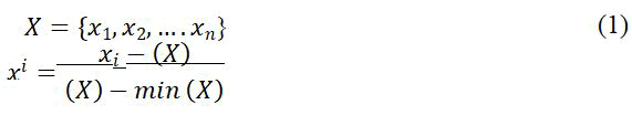
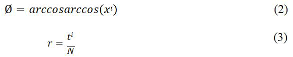
Further, they are transformed into the polar coordinate system using the following equation:

Lastly, the GAF Matrix (G) is obtained from rescaled time series resulting in images fed to the convolutional neural network. Two techniques implemented in this study were Gramian Angular Summation Field (GASF) and Gramian Angular Difference Field (GADF) (Figure 3).

Figure 3: Comparison of normal and schizophrenia Gramian angular fields.

Wavelet transform

The wavelet transform represents an input signal in multiple resolutions using bandpass filters. In a Discrete Wavelet Transform (DWT), signals are categorized into high and low frequency components known as detail and approximation coefficients. Then the approximation coefficients are split into next-level approximate and detailed coefficients and the process continues to depend on the depth of the wavelet tree.

Fourier transform

This transformation decomposes the signal into a series of sine based functions; the absolute values of the Fourier transform represent the signals’ frequency behavior. In this work, Fourier layers were introduced as a starting point for the convolutional neural networks to extract the features from a different representation of the data, which might be more beneficial than the time domain features.

Convolutional Neural Networks (CNN)

CNN is a particular form of neural network commonly used in signal and image processing. CNN utilizes local information by using filters, so-called kernels, which are far more efficient in the number of parameters concerning Multi-Layer Perceptron (MLP). It is the state-of-the-art technique of deep learning to analyze two-dimensional data. A typical set consists of convolutional layers for extracting features, pooling layers to reduce the input dimension and dense layers to map the features into a more distinct space for classification.

Convolutional layers: Convolutional layers apply a linear transformation using a specific kernel. Filters are a way of extracting features from input patterns. The procedure may be described as follows:

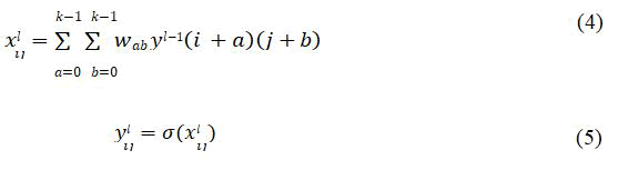
The kernel has a size of K × K, in the case of a symmetrical trainable kernel and the weights are denoted as w_ab. x^l_ij represents an output from the current convolution layer l and y^l-1 shows the last layer’s output, the input to the next layer. Finally, the output y^l_ij is calculated after applying a non-linearity through an activation function chosen as Rectified Linear Unit (ReLU). ReLU is superior to Sigmoid and Tanh due to faster calculation time and better backpropagation in extreme values.

Pooling layers: Pooling layers are a technique to reduce the input size while extracting features with convolutional layers; the most frequent form is called Max Pooling. Where the pixel with the maximum intensity is chosen over each window, reducing the image size to N/K × N/K with a pooling kernel size of K × K. Pooling layers improve the computations in neural networks and provide a method to deal with over fitting by constraining the feature space.

Fully-connected layers: Fully-connected layers also called dense layers, use linear regression-like transformations to give more importance to features that can improve the decision boundary. For example, the procedure is shown below:

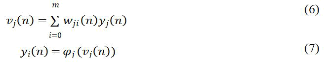
Where y_i is the output of the layer i, computed by multiplying previous layers’ weights w_ji and output y_j, to get v_j(n), then v_j(n) is activated (φ_j), resulting in y_i(n).

Long Short-Term Memory (LSTM)

LSTM, a variant of RNN, preserves the long-term memory of what has been gone through its network. These networks have been introduced to mitigate vanishing gradients from which vanilla RNNs have always suffered. The issue is that the network gradient becomes close to or almost equal to zero before reaching the first layers; therefore, backpropagation becomes less effective. Each LSTM has a cell state vector apart from a hidden state vector to overcome this issue. At each time step, the next LSTM cell can choose to read from its previous cell state, write to it or modify it using four same-shape gates that allow easy information transition and gradient flow through long sequences. These gates are explained in the following sections.

Forget gate: This gate decides whether to preserve information from the previous cell state or forget it. Cell states are the primary components for transmitting information through LSTM cells. This operation can be calculated as equation (8):

Similar to the input gate formula, x_t as input data and h_t-1 as the previous layer’s hidden state is concatenated and fed to a linear transition with w_f and b_f as weights and biases, respectively, eventually, the result is activated using a sigmoid function. The output closer to zero means to forget and one means to retain.

Input gate: The input gate controls whether the cell state is updated by calculating the importance of the current input data to the network. This procedure can be calculated as equation (9):

where x_t is the current input data, and h_t-1 is the previous layer’s hidden state which both are concatenated and passed through a linear transformation with w_i as weights and b_i as biases, finally, a sigmoid function is applied to the previous step, bounding the output between 0 and 1 where the output closer to zero means no update and closer to one means to update.

Candidate gate: Like the input gate, the candidate gate is also responsible for updating the cell state. However, unlike the input gate, this gate performs the Tanh activation function over the linear transformation. Therefore, the expression is simplified into equation (10):

Like the other gates, this gate also feeds concatenated x_t and h_t-1 to a linear transformation with wc and bc presenting unique weights and biases. Finally, the cell state is calculated as in equation (11):

Output gate: This gate controls what percentage of the current cell state’s information should be considered as the final output and transferred as the hidden state to the next cell. This gate can be expressed as equation (12):

Similar to other gates, this gate also conveys concatenated input x_t and h_t-1 and feeds them through a linear transformation and subsequently to a sigmoid activation function while wo and bo featuring unique weights and biases of the linear layer. It is worth mentioning that the current cell state’s information is passed through the tanh activation function before multiplying to the output gate. Thus, the current hidden state and the current cell’s final output are calculated as in equation (13):

FFT-CNN2D

A 19-layer 2D-FFT-CNN model was used in this analysis, as shown in Figure 4, with several parameters in each layer. First, a two-dimensional FFT operation is implemented in the input layer. Then, two convolution operations were conducted in the successive layers, followed by a max-pooling process to extract features from images and reduce their size. A dropout layer also was applied after the mentioned procedures to reduce overfitting possibilities. Following that, for the next round also, two subsequent convolutions were used to construct the following layers (layers 6-7). After the convolutions, the max pooling operation is applied once more to obtain layer 8. Then, to generate layers (9-15), three more convolution and dropout operations were performed alternately. As the next step, the input goes through a flatten layer which converts the vector to a one dimensional format, followed by a dropout layer to reduce over fitting and a dense layer with relu activation to introduce non-linearity. The final layer of the neural network is a dense classification layer with a single output neuron that represents the probability of a given input belonging to either the normal or schizophrenia category.

Figure 4: FFT-CNN2D architecture.

Wavelet-CNN2D

A 2D-wavelet-CNN model was presented in this study, the model architecture is demonstrated in Figure 5, the parameters are also shown in Table 1. First, a two-dimensional Gabor wavelet transform operation was implemented to achieve the first layer’s output. The rest of the structure is identical to the 2D-FFT-CNN. A Gabor filter, introduced by Dennis Gabor, is a linear texture analysis filter in image processing. It examines whether the image contains any specific frequency content in specific directions in a localized region around the point or region of the assessment. A two-dimensional Gabor filter is a Gaussian kernel function induced by a sinusoidal plane wave in the spatial domain.

Figure 5: Wavelet-CNN2D architecture.

Table 1: Models tuning hyper-parameters (identical parameters utilized for all architectures).

Convolutional Neural Network-Long Short-Term Memory (CNN-LSTM)

CNN-LSTM has been gaining much attention in the past few years. It is used on variant tasks like finding spatiotemporal relations in input text for text classification or depressive disorder diagnosis on EEG signals CNN-LSTM results from a series of convolutional layers followed by some LSTM layers. First, it extracts rich features using convolutional layers from input data. Then feeds these features to LSTM layers responsible for extracting temporal information. Finally, the classification is done by applying fully-connected layers to the temporal information obtained by LSTM layers. The CNN-LSTM used in this study consisted of three one-dimensional convolutional layers with a kernel size of 5 and filter sizes of 8, 4 and 2, respectively. Then a dropout layer with a 50% chance of dropping input neurons is applied to avoid over fitting. Following that, a one-dimensional max-pooling layer with a pool size of 2 is applied to reduce the size of the features and consequently, the required computation power. After that, an LSTM layer with a filter size of 512, followed by the second dropout layer with a 25% drop chance, was used. Next, a fully connected layer with 128 units pursued by the third dropout layer with a 25% drop chance was used. Eventually, a fully connected layer with one neuron unit is used to perform classification. All activation functions were ReLU, except for the sigmoid function’s classification layer (Figure 6).

Figure 6: CNN-LSTM architecture.

Transformer

Machine translation was the first application of transformers. In contrast to text data, the signal in the time series is separated into n identical fragments, which is comparable to the embedding procedure on text characteristics. The input data is specified theoretically as follows:

Positional Embeddings have been used in transformers to maintain the order of the series after separation. This layer creates an embedding depending on the maximum length of the segment and the total number of segments. Keys, values and queries are other crucial components of the transformer that aid in the calculation of attention weights; the formula is as follows:

The scaling factor is known as the parameter dk. The multi-head component of the transformer also refers to the fact that the attention’s result is made up of several attention weights, also known as heads, that are merged to learn many input representations in the end. It is also worth noting that for a classification problem only the encoder portion of a transformer is required, with the decoder section being omitted entirely (Figure 7).

Figure 7: Transformer architecture.

Training

First, each signal is converted into an image using GASF and GADF methods for four proposed models. Since there are two measures (GASF and GADF) and 19 different channels, 38 images are obtained for each signal. Figure 2 shows a sample image for healthy subjects and schizophrenia patients. Next, the images are used as inputs of introduced convolutional neural networks. The aforementioned data preparation is the same for transformer-based and CNN-LSTM models, except that the signals are not converted to two-dimensional images and are fed directly to these two models. Finally, f the model training section, a batch size of 4 was selected and each network was trained for two hundred epochs.

Evaluation

Independently, all four proposed models were trained on 80% of the data and then evaluated on the remaining 20%. This procedure was repeated ten times, each time with a distinct initialization setup that was assured with different random seeds. Then the resulting metrics were averaged to derive each model’s mean and standard deviation. The aforementioned metrics were accuracy, sensitivity, specificity and f1-score, which are computed as follows:

Where TP or true positive represents positive samples that are correctly predicted positive, TN or true negative represents negative samples that are correctly predicted negative, FP or false positive represents negative samples that are falsely predicted positive and FN or false negative represents positive samples that falsely predicted negative. Additionally, the initial learning rate was set to 0.0; if there were no improvements after 50 epochs, the learning rate decreased by 0.1. Binary Cross Entropy was chosen as the loss function and in the optimization phase, the ADAM algorithm was chosen due to its superior results and shorter run time. The train-test-split function from the Scikit learn library was used for evaluation.

Results

Table 2 shows the best-obtained metrics over different evaluated deep neural network architectures. Based on this table, the best result is reached by transformer model, which gains the highest average accuracy of 98.50 and a standard deviation of 0.023. The standard deviation value indicates that the model is highly independent of the random seeds used to split the dataset in each run. Transformers' capacity to accurately model the temporal dependencies between input data sequences is the primary factor that may make them more effective than CNNs for some EEG signal classification tasks. Transformers are intended to encode and process sequences of inputs, particularly those with complex temporal structures, in contrast to CNNs, which are primarily made to extract local features from spatially related inputs. To elaborate more on the results, the best confusion matrixes of the models over the evaluation dataset are provided in Figure 5. Accordingly, the transformer model could predict the entire negative and positive samples correctly, resulting in zero FN and zero FP. Likewise, this figure demonstrates the superiority of CNN-LSTM over other models.

Table 2: Models evaluation metrics.

In addition to the transformer model, the CNN-LSTM model has shown a remarkable average accuracy of 95.70 with a standard deviation of 0.0308, the second-best accuracy of the four evaluated models. Moreover, as the corresponding confusion matrix to this model shown in Figure 8 presents, it has two FP and two FN, which is again the second-best confusion matrix compared to the other four models. The other two models, CNN-FTT and CNN-Wavelet, obtain the third and fourth best accuracy of 78.60 and 77.29, respectively. The same results are indicated in Figure 8 for these two models.

Figure 8: Confusion matrix of proposed models.

Discussion

In this experiment, we employed custom deep learning and Gramian Angular Field (GAF) approaches to automate the identification of schizophrenia patients and healthy controls. Our methodology enables automatic feature extraction from time- and frequency-domain EEG information. One of the work’s key innovations is the use of GADF and GASF approaches to transform a 1-D EEG signal into a 2-D representation that can be directly fed to CNN architecture. There are various methods for converting a 1-D signal to a 2-D image, including traditional methods based on time-frequency distribution (STFT, wavelets and so on). Another innovation of the research is using FFT linear and non-linear attributes, demonstrating the superiority of the proposed approach. Additionally, this study has the benefit of comparing various deep-learning models. Ultimately, this research performed better in automatic schizophrenia detection in depressive patients and healthy controls, as seen in Table 3.

Table 3: A summary of previous studies on automated EEG-based schizophrenia detection.

The accuracy of the transformer architecture in images of GADF and GASF methods on 19 channels of EEG signals is 98.5 percent. Furthermore, compared to other deep learning approaches on time-series data of EEG signals, our results with trasnformer and images built with Gramian angular field have higher accuracy compared to other research of this kind. When modeling complex and long-term temporal dynamics for some EEG signal classification tasks, transformer models can yield more reliable and accurate results. According to Table 3, the transformer model outperformed other approaches in terms of accuracy. The findings of this analysis are associated with the new best similar research that used EEG signals from the same database and a separate database and as can be seen, the accuracy obtained in this experiment is higher than that reported in the previous studies using conventional machine learning methods for extracting the networks. The research’s most significant limitation is the scale of the dataset used to train and wavelet layers in the deep model, which processes the input images of the network and creates a time and frequency representation of the EEG signals. We solved this problem by using regularization terms and modifying deep models. Our long-term goal is to extend the experimental area by gathering more data.

Conclusion

A thorough assessment was done in this article using Gramian Angular Field (GADF, GASF) and a variety of well-known deep learning algorithms. The best model is transformer which has the highest accuracy of 98.5% in classifying schizophrenia patients and healthy controls. Traditional convolutional neural networks, which are best for extracting local features and each have a fixed size receptive field, do not adequately model long term dependencies between subsequent input data points. In contrast, the transformer's self-attention mechanism offers a flexible way to choose which parts of the input sequence to emphasize or downplay, enabling it to concentrate on important features across various data scales. Compared to all recent research, this study yielded the best performance. As a result, the new approach will assist healthcare professionals in identifying schizophrenia patients for early detection and treatment.

References

1. Dvey-Aharon Z, Fogelson N, Peled A, Intrator N (2015) Schizophrenia detection and classification by advanced analysis of EEG recordings using a single electrode approach. PLoS One. 2015;10(4):e0123033.

   [Crossref] [Google Scholar] [PubMed]

2. Akar SA, Kara S, Fatma L, Bilgic V. Analysis of the complexity measures in the EEG of schizophrenia patients. Int J Neural Syst. 2016;26(2):1650008.

   [Crossref] [Google Scholar] [PubMed]

3. Dvey-Aharon Z, Fogelson N, Peled A, Intrator N (2017) Connectivity maps based analysis of EEG for the advanced diagnosis of schizophrenia attributes. PLoS One. 2017;12(10):e0185852.

   [Crossref] [Google Scholar] [PubMed]

4. Jahmunah V, Oh SL, Rajinikanth V, Ciaccio EJ, Cheong KH, Arunkumar N, et al. Automated detection of schizophrenia using non-linear signal processing methods. Artif Intell Med. 2019:100:101698.

   [Crossref] [Google Scholar] [PubMed]

5. Zhang L. EEG signals classification using machine learning for the identification and diagnosis of schizophrenia. In 2019 41st Annual International Conference of the IEEE Engineering in Medicine and Biology Society (EMBC) Berlin, Germany, IEEE, pp. 4521-4524.

   [Crossref] [Google Scholar]

6. Buettner R, Beil D, Scholtz S, Djemai A. Development of a machine learning based algorithm to accurately detect schizophrenia based on one-minute EEG recordings. In Proceedings of the 53rd Hawaii International Conference on System Sciences.

   [Google Scholar]

7. Aslan Z, Akin M. Automatic detection of schizophrenia by applying deep learning over spectrogram images of EEG signals. Trait du Signal. 2020;37(2):235-244.

   [Crossref] [Google Scholar]

8. Nikhil Chandran A, Sreekumar K, Subha DP. EEG-based automated detection of schizophrenia using Long Short-Term Memory (LSTM) network. InAdvances in Machine Learning and Computational Intelligence: Proceedings of ICMLCI 2019 2021 (pp. 229-236). Springer Singapore.

   [Crossref] [Google Scholar]

9. Devia C, Mayol-Troncoso R, Parrini J, Orellana G, Ruiz A, Maldonado PE, et al. EEG classification during scene free-viewing for schizophrenia detection. IEEE Trans Neural Syst Rehabil Eng. 2019;27(6):1193-1199.

   [Crossref] [Google Scholar] [PubMed]

10. Oh SL, Vicnesh J, Ciaccio EJ, Yuvaraj R, Acharya UR. Deep convolutional neural network model for automated diagnosis of schizophrenia using EEG signals. Appl Sci. 2019;9(14):2870.

    [Crossref] [Google Scholar]

11. Shalbaf A, Bagherzadeh S, Maghsoudi A. Transfer learning with deep convolutional neural network for automated detection of schizophrenia from EEG signals. Phys Eng Sci Med. 2020;43(4):1229-1239.

    [Crossref] [Google Scholar]

12. Shoeibi A, Sadeghi D, Moridian P, Ghassemi N, Heras J, Alizadehsani R, et al. Automatic diagnosis of schizophrenia in EEG signals using CNN-LSTM models. Front Neuroinform. 2021;15:777977.

    [Crossref] [Google Scholar] [PubMed]

13. Siuly S, Khare SK, Bajaj V, Wang H, Zhang Y. A computerized method for automatic detection of schizophrenia using EEG signals. In IEEE Trans Neural Sys Rehab Eng. 2020;28(11):2390-2400.

    [Crossref] [Google Scholar]

14. Olejarczyk E, Jernajczyk W. Graph-based analysis of brain connectivity in schizophrenia. PLoS One. 2017;12(11):e0188629.

    [Crossref] [Google Scholar] [PubMed]

15. Zhang G, Si Y, Wang D, Yang W, Sun Y. Automated detection of myocardial infarction using a gramian angular field and principal component analysis network. IEEE Access. 2019;7:171570-171583.

    [Crossref] [Google Scholar]

16. Xu H, Li J, Yuan H, Liu Q, Fan S, Li T, et al. Human activity recognition based on gramian angular field and deep convolutional neural network. IEEE. 2020;8:199393-199405.

    [Crossref] [Google Scholar]

17. Islam MM, Shuvo MM. DenseNet based speech imagery EEG signal classification using Gramian Angular Field. In2019 5th International Conference on Advances in Electrical Engineering (ICAEE) 2019, Dhaka, Bangladesh, IEE, pp. 149-154.

    [Crossref] [Google Scholar]

18. Saeedi A, Saeedi M, Maghsoudi A, Shalbaf A. Major depressive disorder diagnosis based on effective connectivity in EEG signals: A convolutional neural network and long short-term memory approach. Cogn Neurodyn. 2021;15(2):239–252.

    [Crossref] [Google Scholar] [PubMed]

19. Saeedi M, Saeedi A, Maghsoudi A. Major depressive disorder assessment via enhanced k-nearest neighbor method and EEG signals. Phys Eng Sci Med. 2020;43(3):1007–1018.

    [Crossref] [Google Scholar] [PubMed]