Fisheries and Aquaculture Journal
Open Access

Maximum Likelihood Estimation of Kokanee and Sockeye Salmon Spawners in a Stream Using Visual Survey Data, 2003-2017

Marc Labelle, Richard Bussanich^* and Ryan Benson ^*Correspondence: Richard Bussanich, Department of Okanagan Nation Alliance, West Bank, Canada, Email:

Author info »

Introduction

Kokanee, a smaller lacustrine relative of anadromous Sockeye Salmon (Oncorhynchus nerka) rear in Skaha Lake (BC) and mostly spawn upstream in the Penticton Channel. In 2009, the McIntyre Dam that blocked upstream passage of Sockeye salmon since 1954, was improved to provide upstream passage. Hatcheryreared Sockeye released in the Okanagan River since then started returning via the Columbia River in 2011 to Skaha Lake and can also spawn in the channel. Spawner abundance was systematically monitored since 2003, but the arrival of Sockeye complicated assessments due to differences or overlap in arrival times, survival patterns, size distributions and the presence of hybrids (Figure 1).

Figure 1: Location of the Penticton Channel and the 6 section boundaries used for visual surveys were conducted during 2003-2017 for kokanee and Sockeye salmon.

Additional monitoring began in 2011 to determine the kokanee: Sockeye ratio by means of mark-recapture, dead-pitch surveys, bio-sampling, and genetic analyses [1]. These investigations were logistically complex, labor intensive, expensive, and could not be justified in the long run. A priority was developing an alternative assessment procedure that visual survey records for both Nerkids with information from complementary investigations.

Based on habitat type, the channel was initially divided into 6 sections in lengths ranging from 280-740 m, with average depth of <10 m. Section 6 is a low flow and deeper area that lacks suitable spawning areas because of large beds of Eurasian water milfoil (Myriophyllum spicatum). So kokanee simply hold there before spawning or move back to Skaha Lake. Since 2003, visual surveys were conducted 1-3 times a week by two experienced observers from an inflatable raft. Kokanee tend to spawn in large aggregations, and easily recognized by small body and brilliant reed coloration. However, visual surveys are less effective with increased spawning period as coloration is less pronounced. Numbers of live and dead fish are recorded in all sections. During 2003-2010, spawner abundance was mainly estimated using the area-under-thecurve method. Alternative estimates were made in some years using peak-to-peak methods and the Millar and Jordan Gaussian areaunder- the-curve method [2-4].

The limitations of traditional area-under-the-curve type estimators are well-known. Many are described by Perrin and Irvine [2]. These are often related to stream life (or survey life), survey timing, observer efficiency, and implicit hypotheses. After examining the 2003-2017 survey records, it was reasoned the maximum likelihood model for visual surveys might suitable for the present context because (i) it as peer reviewed and published, (ii) it uses live counts not always covering the during peak abundance period; (iii) it can provide estimates of observer efficiency and stream life, (iv) it can used ancillary data to suit the peculiarities of different systems, and (v) confidence intervals can be generated from likelihood profiles [5-7].

The Hilborn et al. model is suitable for a single-species context that has one major mode. Labelle and McHugh proposed a bi-modal version of it that better accounts for salmon escaping to small coastal streams subject to a first and a second larger freshet. That model was adjusted here to account for two Nerkids that do have the same stream occupancy pattern. So variants of the uni-modal and bi-modal models were developed for this context [6,8].

Materials and Methods

Model notation

i   variable denoting a time index (in days, range: 0 to t_max)

j   variable denoting the number of days in a given interval (1 to max=J)

k   variable denoting the day number for a given time interval

m    variable or subscript denoting a mean arrival time

n   variable denoting the number of observations (or sample size of n)

p   variable denoting the probability of an event

r   variable denoting successes in a negative binomial model

s   variable denoting the number of days spawners survive in the channel

s̅   variable denoting the average of stream life estimates over several seasons

t   subscript denoting successive days (0-108 for Aug. 15-Dec. 1)

v   variable denoting an index of seasonal observer efficiency

c_t   variable denoting the expected number of live fish count, time t

x_t    variable denoting the actual count of live fish, time t

y   subscript denotes a year

df   degrees of freedom, i.e. difference in parameters of the models compared

σ   standard deviation

A_t   variable denoting the cumulative number of arrivals, time t

D_t   variable denoting the cumulative number of deaths, time t

E   variable denoting the total number of fish entering a stream

E_t   variable denoting the number of salmon entering a stream at time t

N_t   variable denoting the number of live fish potentially observable, time t

P   cumulative probability of an event given a model

L   Likelihood

ℓ   Log-Likelihood

   Likelihood ratio

α   shape parameter (alpha) of the Weibull distribution

β   scale parameter (beta) of the Weibull distribution

Φ   proportion of kokanee in total spawners

Γ   gamma function

θ_h   vector of parameters values for hypothesis h

x   vector of actual counts for a given stream/season

Data records and survey conditions

All survey records are stratified by year, survey period, and fish condition (live, dead). Survey conditions are reported but are more qualitative than quantitative. These include indices of turbidity, visibility, luminosity levels, cloud cover, wind strength, with notes on potential shadowing (shallow fish over deeper fish) and carcass removal rates. Survey records considered to be problematic were removed before assessment. They consist mainly of survey counts obtained under detrimental conditions, as when luminosity level is low, winds are high, water is turbid or there is evidence of shadowing as when fish are stacked on top of each other. The number of usable survey records for assessment ranged from 8-14 per season between September 20 and December 5.

Model structure

The model described uses a notation similar to that of Hilborn et al. [6]. Their model uses arrival and departure functions based on the normal distribution. Arrivals consist of the cumulative number of live fish that enter the stream. Departures consist of the cumulative number of dead fish, a function of stream life. Omitting the stream and year subscripts for purposes of clarity, the arrival and departure functions are:

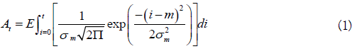
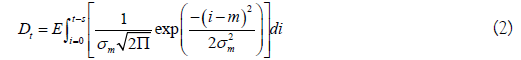
In the above, the fish alive on a given day is given by A_t-D_t, using a constant and time-invariant stream life value (s). The arrival of kokanee or Sockeye on the spawning grounds may not be normally distributed, so a Weibull distribution was used as an alternative. For a fixed stream life (s), Eq. 1-2 become

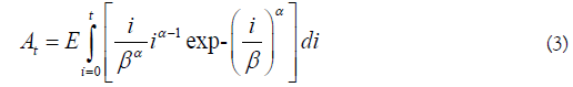
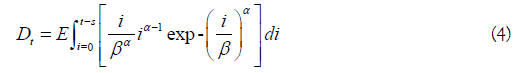
In Eq. 3-4, alpha and beta are shape and location parameters. If alpha>beta, the distribution is left skewed, and the opposite if alpha<beta. The arrival time mean and standard deviation are respectively given by βΓ(1-α^-1) and β²[Γ(1+2α^-1)-Γ²(1+α^-1)].

Modified departure functions

Labelle noted that tagged Coho escaping to small coastal streams had skewed stream residency patterns, and used a Log-normal distribution for survival applicable to daily pulses of immigrants [9]. Replacing the constant stream life by survival probability distribution requires formulating alternative departure functions (Eq. 2,Eq. 4).

The simplest survival model used tried is a Poisson distribution, with a mean equal to the variance both denoted by s. If s=10 d, stream life ranges from 2-22 d, so some die 2 days after entering the stream, most die after 10 day, and some live 22 days. Let the stream residency period be denoted here by j1 to j_max=J=22. The probability that a fish is dead j days after entering the spawning area is given by the Poisson cumulative distribution

For all fish entering a stream at a given day (Et), the proportion dead by time t+j is computed from Eq. 5 to determine the totals deaths on a given day as Eq. [6], Eq. [7] and Eq. [8].

The Poisson probability model can cause over-dispersion when the variability in the data is greater than the model predicts. The Negative Binomial distribution was used as an alternative since it can be positively skewed (like a Log-normal). This distribution has a variance ≥ mean, and can account for non-symmetrical stream life patterns as when males survive longer than females. It is computed from the probability of j failures before the r^th success, with each Bernoulli trial with a probability of success p. The Negative Binomial cumulative probability distribution is

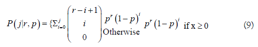
Eq. 9 is the probability that a fish is dead j days after entering the spawning area. To use the Negative Binomial model instead of the Poisson model, just substitute P(j|s) by P(j|rp) in Eq. 5 and Eq. 7 and re-compute for The mean and standard deviation of stream life are computed from s=(r(1-p))/p, an σ_s=(r(1-p))/p².

Using these functions imply that all groups of fish entering the spawning ground on given days are subject to the same survival pattern from the date of entry. The arrival-departure trends based on the Normal-Poisson yield two cumulative distributions offset by the average stream life (Figure 2).

Figure 2: Example of the cumulative abundance trends for live and dead kokanee (solid and dashed lines) estimated with a Normal-Poisson model. The two abundance trends are offset by the estimated stream life (vertical double-pointed line).

Observer efficiency

Irrespective of the arrival-departure function chosen, the expected number of salmon alive at time t that may be seen by observers (c_t) is usually computed using observer efficiency measurements (v_t). Observer efficiencies are not measured during the channel surveys, and only crude indices are reported. The Hilborn et al. model is well-suited since it uses a scaling coefficient, considered somewhat akin to a seasonal average or the best-fitting value in a maximum likelihood context [6].

The above computations (Eq. 10 and Eq. 11) serve to provide vectors of observed and expected counts by survey day. The two vectors are used to estimate spawner abundance, arrival times, observer efficiency and stream life.

Fitting the model to data

Surveys counts are for kokanee up to 2010 and both Nerkids after. Field observations indicated the two Nerkids do not have identical patterns of stream occupancy. The bi-modal model of Labelle and McHugh [8] has an extra parameter for the kokanee: Sockeye ratio, and two sets of run timing and stream life parameters. Single observer efficiency is used for joint monitoring of Nerkids with overlapping sizes. Let the fraction of kokanee in total spawners be denoted by Φ. The uni-modal and bi-modal models tried were

Normal-Poisson, with parameter set θ₁₌{E,m,σ_m,s,v}.

Normal-NegB, with parameter set θ₂₌{E,m,σ_m,r,p,v}.

Weibull-Poisson, with parameter set θ₃₌{E,α,β,s,v}.

Weibull-NegB, with parameter set θ₄₌{E,α,β,r,p,v}.

Weibull-Poisson bi-modal, with parameter set θ₅₌{E,Φ,α₁,β₁,s₁,α₂,β₂,s₂,v}.

Weibull-NegB bi-modal, with parameter set θ₆₌{E,Φ,α₁,β₁,r₁,p₁,α₂, β₂,r₂,p₂,v}.

Parameter estimation

Hilborn et al. estimate parameters in the absence of known process error, the objective function mainly accounts for observation error [6]. The authors noted that variance in observer counts tended to increase with abundance in their context, and modelled observation error after a pseudo-Poisson distribution with a variance scaled by coefficient (q). Examination of repeated or temporally close observer counts provided no evidence that variance in counts increased non-proportionally with abundance. For the Poisson distribution, the variance is equals the mean so the increase is proportional. Observed and expected frequencies of Poisson distributed events by category (survey period) are often compared using likelihood-ratio tests when expected frequencies are relatively large. According to Baker and Cousins, the appropriate statistic for comparison of Poisson events is Neyman’s The authors note that minimization of is entirely equivalent to maximization of the likelihood function, and can be used for both testing and maximum likelihood estimation. They define the Poisson Likelihood chi-square as

Ross uses a nearly identical but equivalent function that yields the same results. Eq. 12 is basically a log-likelihood ratio statistic because logarithms are used. Eq. 12 is a Likelihood function that expresses the probability of a hypothesized set of parameter values given the observation data vector. Using Edwards conventional notation;

Eq. 13 is the objective function used as the observation error model and fitting criterion to estimate the best parameter values. This is obtained by maximizing theL(θ_h), with the best estimate denoted by [10-13].

Adjustments for uncertainties

Hilborn et al. adjusts the likelihood function when prior information is available. The example given has Normal Likelihood functions for escapement, stream life and observer efficiency. The overall Likelihood is the product of 3 likelihoods. In the present context, the few historical stream life values do not conform to any parametric distribution, and there are no measurements of observer efficiency, so this approach was not used. Instead, priors and bounds were based on a mix of field observations, complementary investigations, model-based estimates, and surveyor reports [6].

Bounds prevent the function optimization algorithm from “converging to a solution in the unrealistic range of the parameter space”. Bounds were set to values considered plausible. The lower bound for total abundance is the maximum survey count, average stream life is 5-14 days for both Nerkids, and observer efficiency is 0.70-0.95. Lower bound for arrival time and maximum stream residency is based on survey counts. Bounds for the proportion of kokanee in spawners were set by a committee of regional biologists working on the system, based on mark-recapture results, Nerkid composition in dead-pitch surveys, and genetic analyses of biosamples. This is akin to using ‘expert-based’ priors in a Bayesian estimation context [14,15].

Confidence intervals of spawner abundance

Ross notes the critical contour for likelihood profiles is often given by with 95% confidence intervals based on α=0.05 and df=1, for an interval of 3.841. Lower and upper confidence intervals are given by the likelihoods for hypotheses for 0.5 χ² or 1.92 units away from the maximum likelihood. Some prefer 95.4% confidence limits so 2.0 units away. The best and alternative hypotheses are often compared with log-likelihoods so 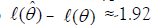which is the procedure used here. For likelihoods use L(θˆ)/ L(θ ) ≈exp(- 1.92) ≈ 0.147. A likelihood profile for abundance is obtained by sequentially computing L(θ ) for increasing and decreasing abundance values, while searching for the best combination of the remaining ‘nuisance parameters’. The lower and upper intervals are the smallest and greatest abundance estimates of the profile [12,13].

Results

The bi-modal model fits survey records well even when one apparent peak is minor (Figure 3). Since minor counts <0.5% of the peak counts were discarded, the survey series for all years had a single peak count and one obvious mode. Only the uni-modal models were used analyse the kokanee only records of 2003-2010. The Normal-NegB model provided better fits than the Normal- Poisson. The Normal-NegB and Weibull-NegB fits were similar (Figure 4), but the later was better since the Normal-NegB model did not fit early or late survey counts as well. Akaike’s Information Criterion (AIC) tests were not use to compare models given the same number of parameters. Likelihood ratios tests confirmed the Weibull-NegB models were way better. And since it was also more versatile, the entire 2003-2017 series where fitted with the Weibull- NegB models [16].

Figure 3: Example of a Normal-Poisson bi-modal model fit to kokanee survey records with two modes. The expected values conform to the survey counts well even when a hypothesized second mode is relatively small.

Figure 4: Fits obtained with the uni-modal model version for 2007 kokanee spawner abundance. The Normal-NegB model (top) and the Weibull-NegB model (below).

The bi-modal version accounts for the underlying distributions of abundance of both Nerkids in the total expected abundance trend for 2014 (Figure 5). Unless the underlying abundance trends differ temporally, the total trend may not appear to be bi-modal. In 2014, the stream life distributions of kokanee and Sockeye were very similar, but the arrival distributions differed considerably, with Sockeye arriving on the grounds later over a much narrower period (Figure 6). Similar trends were obtained for other years. One potential explanation is that Sockeye hold for weeks in Skaha Lake without eating, and only move to spawn at times based on energy reserves. By contrast, kokanee can forage all the time before the spawning period. The estimates obtained provide some support for the notion that kokanee enter the spawning grounds later and stream life is shorter under low stream temperature (Figure 7).

Figure 5: Expected abundance trends for kokanee and Sockeye combined (thick line), fitted to the 2014 survey counts (dots) by survey day number (x axis) with the Weibull-NegB models. Underlying expected trends for kokanee (dashed) and Sockeye (smaller dash). Kokanee accounted for 62% of the run, with kokanee abundance peaking a few days before Sockeye.

Figure 6: Estimated probability distributions of stream life (x-axis values) for kokanee (top left) and Sockeye (top right) for 2014. The probability distributions for arrival time (x-axis values) are in lower 2 graphs in same order. The 90% confidence interval values are given above each graph. Streamlives were similar, but Sockeye enter the spawning grounds later over a much narrower period.

Figure 7: Estimated peak run day versus measured stream temperatures in Oct.-Nov. for kokanee during 2003-2006 and 2008-2017 (top). Estimated mean stream life versus average stream temperature (bottom). Linear regressions given for visual reference purposes only.

Kokanee spawner abundance was relatively stable over 2003- 2017, with a high in 2007 and a low in 2013 (Table1). Observer efficiency mostly in the 0.80-0.90 range, never <0.71 or >0.92. Average kokanee stream life was 6-12 days with few exceptions. Sockeye contributions were 0.06-0.38 of total abundance since 2011 (median≈19%) with low contributions in 2015-2016 because adult returns were reportedly subject to low ocean survival rates.

Table 1: Estimates based on the trapezoid method (Col. 1), the Gaussian method (Col. 2-3) and the Maximum Likelihood method (Col. 4-12). Gaussian estimates are for live + dead kokanee sections 1-6 with observer efficiencies of 1.0. Peak run time, stream life and observer efficiency estimates from Maximum Likelihood model based on live counts in sections 1-5. Day number and corresponding dates given for reference purposes.

Spawner examination showed that some kokanee are large and many have gill-net marks likely from Columbia River fishery interceptions. Genetic testing confirmed these were kokanee hybrids that switched to an ocean-going Sockeye life history. Hybrids genetically determined to be Sockeye were small with no gill-net marks, and likely switched to a fresh-water lifestyle. The kokanee proportion estimate may account well for the two life history types but more testing is needed to confirm that, and determine if Sockeye hybrids pair up with kokanee.

Confidence intervals of spawner abundance

The Gaussian AUC model was not used to estimate the respective abundances of kokanee and Sockeye when both were present. An independent assessment done in 2005 yielded estimates of abundance and confidence intervals of ≈79000 and 35,000- 130,000. Those computed with the Weibull-NegB model were similar so ≈79,500 and 31,000-118,000 (Figure 8). The approximate lower interval limit (31,000) is less than the peak survey count (41,000). If penalty functions were used to reduce the influence of large residuals, the penalize likelihood profile could be narrower, unsymmetrical, and not cover the maximum count [9].

Figure 8: Likelihood profile for kokanee spawner abundance in 2005. Approximate 95% confidence intervals are abundance levels where the profile crosses the x-axis at value -1.92, so ≈31,000-118,000. The best abundance estimate is at the peak y-axis value of 0.0 vertically offset lightly to improve readability.

Discussion

Confidence intervals obtained for other years are not reported here for purposes of brevity. Those for years with kokanee and Sockeye present will be revised in light of the results from on-going monitoring. For most years, there are no alternative abundance estimates or fence counts to serve as accurate reference points for comparative purposes. There are more complex area-under-thecurve type estimators of escapement for data-rich contexts [17]. But for this simple and data-poor context, efforts focused on developing a model better than the ‘trapezoid’ model and suited for a two Nerkid system. The present model can be implemented in MS Excel using methods described in [18]. This is useful for users not well-versed in C++ or VBA programming, or expertize with modelling platform languages such as R, Win BUGS and AD Model Builder. The results obtained so far are comparable not very different than the few obtained in other investigations. The present approach provides a consistent way to analysing the entire 2003-2017+ data series, and may be considered sufficiently good current annual monitoring and stock management purposes

Unfortunately, the accuracy and precision of the estimates obtained cannot be determined with certainty at this stage. Conducting complementary investigations would be helpful, even if done on a periodical basis. Electronic monitoring of movement into the spawning channel by means of ARIS imaging sonars, resistivity counters and counting towers might provide consistent and useful escapement indices without causing mortalities or relying on labor intensive field operations. Further insight into observer efficiency might possibly be obtained by having a diver with snorkelling gear accompany the boat, do counts and measure observer visibility ranges. Future surveys and model-based estimates are needed to help determine the alternative assumptions needed to improve the models described, provide additional data to set priors, bounds and penalty functions.

Information provided from assessments and on-going monitoring is important to justify continued efforts to re-introduce Sockeye into Canada and support Columbia River fisheries. The reintroduction and the potential impact on kokanee are subject to considerable scrutiny by Canadian scientists, and long-long monitoring is recommended to ensure that bio-diversity is not negatively impacted. The benefits of Canadian Sockeye production returns to the Columbia Basin (last 10 years 80% of total returns) should be sustained and even improved [19].

Conclusion

At this stage, there is no evidence from assessment or surveys that kokanee spawners are negatively impacted by Sockeye that have a later and narrower spawning window. Sockeye may have slightly different spawning substrate preferences, so the small spatialtemporal segregation may explain the lack of [obvious] impacts. Further monitoring is needed to ensure that both Nerkids can co-exist, do not interfere with each other, or cause hybridization to reach problematic levels. Monitoring would also provide more information on the channel capacity to support higher spawner densities and where habitat improvements could be made.

Harvest strategies are an integral part of Stock reintroduction programs. Currently, harvesting is not allowed in Shaha Lake, although goals have been set for the First Nation Food, Social and Ceremonial Fishery, and the multi-species inland recreational fishery. Establishing spawning escapement targets is necessary before harvest limits are set. Based on habitat capacity estimates, the current interim spawner target proposed by the Okanagan Nation Alliance for Skaha Lake (excluding Osoyoos Lake) are 3000 Sockeye and 21,000 kokanee, the geometric mean escapement in 4 of a 5 year period. It also requests that US allows 60,000 Sockeye to reach Priest Rapids dam, and 100,000 during 10 d periods of warm water (>20 oC). This is substantially greater than the current Pacific Salmon Treaty agreement target of 30,000 Sockeye. Future fishery management plans should ensure ONA targets are met to justify continued hatchery production from its Penticton facility. Ongoing monitoring, assessments and investigations such as this one can help meet such objectives.

Acknowledegements

The Okanagan Nation Alliance (ONA) that facilitated this project would like to thank the Penticton Indian Band for their support and allowing us access to sampling sites. Funding was provided by Grant and Chelan County Public Utility Districts (Washington State). We would like to thank the following ONA staff for their contributions: Casmir Tonasket, Dave Tom, Saul Squakin, Nicholas Yaniw,and Colette Louie (Osoyoos Indian Band).Last but not least is the support of Howie Wright,ONA Fisheries Program manager, who helped coordinate and justify this investigation.

References

1. Bussanich R, Benson R, Friesen A. qawstik’wt [Skaha Lake] Kokanee Spawner Enumeration and Biological Sampling 2010. 2013.
2. Irvine JR, Bocking RC, English KK, Labelle M. Estimating coho salmon (Oncorhynchus kisutch) spawning escapements by conducting visual surveys in areas selected using stratified random and stratified index sampling designs. Can J Fish Aquat Sci. 1992;49(10):1972-1981.
3. Skalski JR, Liao S, Buchanan RA. Performance of three alternative estimators of stream residence time based on live and dead counts of salmonids. N Am J Fish Manag. 2010;30(1):191-208.
4. Millar RB, Jordan CE. A simple variance estimator for the trapezoidal area-under-the-curve estimator of the spawner abundance of Pacific salmon. Can J Fish Aquat Sci. 2013;70(8):1231-1239.
5. Perrin CJ, Irvine JR. A review of survey life history estimates as they apply to the area-under-the-curve method the spawning life escapement of Pacific salmon. Can Tech Rep Fish Aquat Sci. 1990.
6. Hilborn R, Bue BG, Sharr S. Estimating spawning escapements from periodic counts: a comparison of methods. Can J Fish Aquat Sci.1999;56(5):888-896.
7. Korman J, Ahrens RN, Higgins PS, Walters CJ. Effects of observer efficiency, arrival timing, and survey life on estimates of escapement for steelhead trout (Oncorhynchus mykiss) derived from repeat mark recapture experiments. Can J Fish Aquat Sci. 2002;59(7):1116-1131.
8. Labelle M,   D. McHugh, 2014. Investigation of chinook escapement survey and estimation methods for West Coast Vancouver Island (WCVI) streams. Can Sci Advis Sec Res. 2014;62.
9. Labelle M. A likelihood method for estimating Pacific salmon escapement based on fence counts and mark–recapture data. Can J Fish Aquat Sci. 1994;51(3):552-566.
10. Baker S, Cousins RD. Clarification of the use of chi-square and likelihood functions in fits to histograms. Nucl Instrum Methods Phys Res.1984;221(2):437-442.
11. Edwards AW. Likelihood. Expanded edition Johns Hopkins University Press. Baltimore, 1992.
12. Bard Y. Nonlinear parameter estimation. Academic Press, New York, 1974;p:341.
13. Morris PA. Combining expert judgments: A Bayesian Approach. Manage Sci. 1977;23(7):679-693.
14.  Akaike H. Information theory and an extension of the maximum likelihood principle. In Selected papers of hirotugu akaike. Springer, New York, 1998;pp:199-213.
15. Korman J, Melville CC, Higgins PS. Integrating multiple sources of data on migratory timing and catchability to estimate escapement for steelhead trout (Oncorhynchus mykiss). Can J Fish Aquat Sci. 2007;64(8):1101-1115.
16. Haddon M. Modelling and quantitative methods in fisheries. CRC press, 2010.
17. DFO. Review of potential impacts associated with recent and proposed Okanagan Sockeye salmon fry introductions to Skaha and Okanagan Lakes. Can Sci Advis Sec Sci Resp. 2017.