Fisheries and Aquaculture Journal
Open Access
ISSN: 2150-3508
ISSN: 2150-3508
Research Article - (2016) Volume 7, Issue 2
We developed an in-season forecast model of return of chum salmon for the population off the Honshu region in the Sea of Japan using the smoothing spline based on catch data obtained in fishing season. The optimal in-season model was constructed using adult return in season 8 (middle October) as an explanatory variable. Residual sum of squares of the optimal in-season model was lower than that of the pre-season forecast (sibling) model, indicating the former was more accurate than the latter. The relationship between forecast error rate in the optimal model and the cumulative proportion of return until season 8 (middle October) was positive. Yearly variation in the forecast error rate may be affected by variability in the timing of return. We provide a new and accurate forecast model of chum salmon return.
Keywords: Chum salmon, Forecast, GAM, In-season, Oncorhynchus, Pacific salmon, Sibling, Sea of Japan, Smoothing spline
Mature (adult return) chum salmon (Oncorhynchus keta) migrate from offshore into coastal waters and natal rivers to breed [1,2]. Spawning season spans approximately 7 months, from August to February [3]. In Japanese waters, returning adults are caught mainly by set-nets in coastal waters off natal rivers, and by gill- and purse-seine nets within rivers. Therefore, the number of returning adults is defined as the sum of numbers caught coastally (coastal catch) and numbers caught in rivers (river catch). As the fishing season proceeds the cumulative proportion of returning adults gradually increases (Figure 1). We can view in-season catch data as a kind of relative density index obtained by in-season survey.
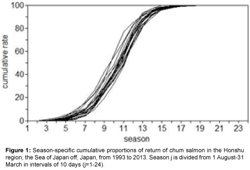
Figure 1: Season-specific cumulative proportions of return of chum salmon in the Honshu region, the Sea of Japan off, Japan, from 1993 to 2013. Seasonj is divided from 1 August-31 March in intervals of 10
At present, the pre-season forecast model of Japanese chum salmon, which is the sibling model, it has been often used to forecast agespecific return number. This pre-season forecast model requires many biological parameters and assumptions, which are age composition and constant rate of maturation through study period. Whereas, inseason forecast model using only in-season catch information could require no parameters and assumptions (Figure 1). In addition, a nonparametric approach such as smoothing spline is expressed with the added advantage of not having any a prior assumption of linearity [4]. Several studies have developed nonparametric models for inseason forecasts [5,6]. In-season forecast model using catch data and smoothing spline could ensure simplification of forecasting.
The in-season model in this study does not consider variability in salmon return timing, which is affected by both genetic and environmental factors [7,8]. The return timing affecting in-season catch, return, and the cumulative proportion of the adult return (Figure 1) could cause forecast error of the in-season model. We focused on the relationship between forecast error rate and the cumulative proportion of the adult return.
The purpose of this study was to develop in-season forecast models for chum salmon return by using smoothing spline. We compare forecast accuracy of the in-season forecast model with that of preseason forecast model.
Study area and population
In this study, we subject data to the chum salmon population in the Sea of Japan off the Honshu region, Japan to forecast models (Figure 2). This regional population includes river stocks of chum salmon in the region (Figure 2). The region includes coastal areas in Aomori, Akita, Yamagata, Niigata, Toyama, and Ishikawa Prefecture.
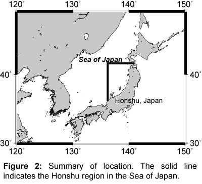
Figure 2: Summary of location. The solid line indicates the Honshu region inthe Sea of Japan.
Data source
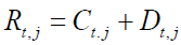
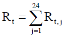
The coastal catch in number, C, and river catch in number, D, in the regional population of the Sea of Japan off Honshu were used for 1993-2013 [9]. The catch data were collected by Aomori, Akita, Yamagata, Niigata, Toyama, and Ishikawa Prefecture. The catch data were summarized each season j (1st season is 10 days). The season j-specific return, Rt,j, and the total return in year t were defined as:
 (1)
(1)
 (2)
(2)
where j is the season that is divided from 1 August-31 March in intervals of 10 days (j=1-24). For example, j=1, 2 and 3 represent periods from 1 to 10 August, 11 to 20 August, and 21 to 31 August, respectively.
Smoothing spline model
To evaluate relationships between log-transformed total return Rt and catch data in-season, models were constructed for the following four cases:
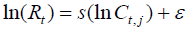 (3)
(3)
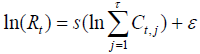 (4)
(4)
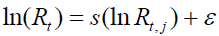 (5)
(5)
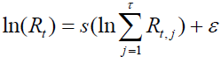 (6)
(6)
where s is the smoothing spline function and ε is assumed to be normal distribution. Function s is estimated by minimizing penalized residual sum of squares and equivalent 4 degrees of freedom in GAM by using S+ version 8.1 [10]. In Equations (3-6), explanatory variables are coastal catch, Ct,j, cumulative coastal catch-to-date, ΣCt,j, return Rt,j, and cumulative return-to-date, ΣRt,j, separately. In addition, to test explanatory variables in various fishing seasons, we used variables from fishing starting season 1 to 8 when the cumulative proportion of adult return met 0.5 (Figure 1). However, in seasons 1-5, return and catch were frequently 0. Therefore, to avoid values of 0 as explanatory variables, we used variables in seasons 6,7 and 8. Thus, season j was given as 6,7 and 8 in the case of Equations (3) and (5). In the case of Equations (4) and (6) τ is given as 6,7 and 8. Therefore, we generated 3 models for each case. The total number of models was 12 (Table 1).
| Model | Explanatory variable | Season |
|---|---|---|
| 1 | Ca | 6 |
| 2 | C | 7 |
| 3 | C | 8 |
| 4 | Cumulative C | 1-6 |
| 5 | Cumulative C | 1-7 |
| 6 | Cumulative C | 1-8 |
| 7 | R | 6 |
| 8 | R | 7 |
| 9 | R | 8 |
| 10 | Cumulative R | 1-6 |
| 11 | Cumulative R | 1-7 |
| 12 | Cumulative R | 1-8 |
| 13 | Sibling | Pre-season |
Table 1: In-season forecast models and sibling model. Coastal catch (C) and return (R) of chum salmon.
In-season forecast procedure by cross-validation
Fitting of the above models is a part of forecast procedure. Logtransformed R was forecast by the following cross-validation:
Step 1: A smoothing spline was estimated by GAMs using data from 1993 to t, indicating fitting of the models (Equations: 3-6).
Step 2: An explanatory variable in t+1 is substituted into the estimated models and then ln(Rt+1) is forecast.
This procedure was repeated from t=2000 to 2012. Therefore, yearspecific forecasts, ln(Rt+1), were provided for each year from 2001 to 2013.
To evaluate the accuracy of model forecasts, the residual sum of squares (RSS) was measured for each in accordance with:
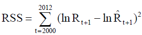 (7)
(7)
In addition, forecast error rate was calculated for each year. Note that the cumulative proportion of the adult return for any given season varied between years (Figure 1). Thus, the forecast error rate may be affected by return timing. We investigated relationships between forecast error rate and the cumulative proportion of returning adults.
Pre-season forecast
The sibling model, a traditional pre-season forecast model, was used to forecast the number of adult returns for specific age classes, as follows:
Step 1: Linear regression of log-transformed R at age a-1 in t-1 against log-transformed R at age a in t is estimated by using data from 1993 to t as:
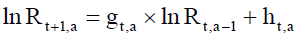 (8)
(8)
where gt,a is the regression slope and ht,a is the intercept from 1993 to t at ages a from 3 to 7. Calculations for 5 ages classes over 13 years produced 65 regressions. Note for ages 2 and 8 a regression (Equation 8) cannot be estimated. At ages 2 and 8, forecast values are given as the average of observed ln(Rt,2) and ln(Rt,8) from t to t-4, separately.
Step 2: When gt,a is significant (p<0.05), an explanatory variable, i.e., return at age a-1 in t, is substituted into the estimated regression (Equation 8) and then ln(Rt+1,a) is forecast. If gt,a is not significant (p<0.05), ln(Rt+1,a) is given as the average of observed ln(Rt,a) from t to t-4. Finally, age-specific forecasts ln(Rt+1,a) were combined by year. Age-combined forecast, ln(Rt+1), were calculated for each year from 2001 to 2013.
This procedure was repeated from t=2000 to 2012. RSS between actual ln Rt+1 and age-combined lnΣ(Rt+1,a) was calculated using Equation (7).
In catch models 1,2 and 3, RSS decreased as the season progressed from 6 to 8 (Figure 3). In cumulative catch models 4,5 and 6, and in return models 7,8 and 9, RSS also decreased in the same manner with catch models. To the contrary, in cumulative return models 10,11 and 12, RSS decreased as the season proceeded from 6 to 7 but increased in season 8. Of all 12 in-season models (Table 1), catch model 3 had the lowest RSS (Figure 3). RSS in model 3 was lower than that of the sibling model 13, indicating that, of all models examined, the optimal model was catch model 3.
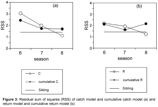
Figure 3: Residual sum of squares (RSS) of catch model and cumulative catch model (a) and return model and cumulative return model (b).
The optimal model was particularly good at forecasting variation in the observed return in 2004-2008 compared with the sibling model (Figure 4). Ability of forecast the return of the optimal model (catch model 3) was better than that of the sibling model (Figure 3). Therefore, our result provides a new, simple, and accurate in-season forecast model compared with the sibling model.
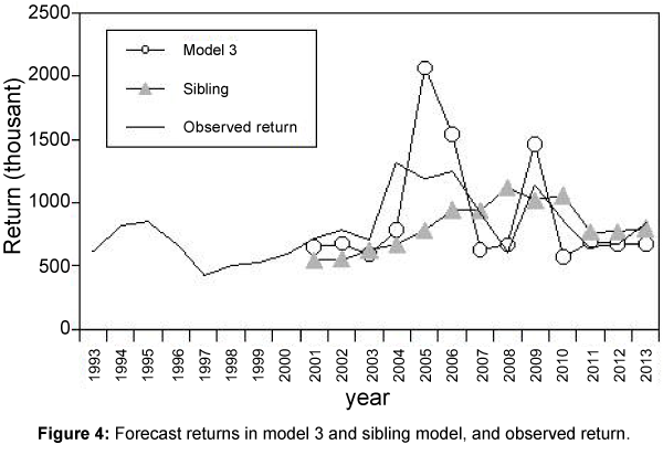
Figure 4: Forecast returns in model 3 and sibling model, and observed return.
The relationship between forecast error rate in catch model 3 and the cumulative proportion of return until season 8 (middle October) was positive (Figure 5). Yearly variation in the forecast error rate may be affected by variability in the timing of return [7,8]. Further study would need to incorporate variables associated with variability in the return timing into in-season forecast model. However, the forecast error rates of catch model 3 were relative low. In addition, smoothing splines of catch model 3, which were estimated by GAM framework, were soaring curves against coastal catch in season 8 (Figure 6). Although the end year for modeling, i.e., year t, changed from 2000 to 2012, the form of these curves did not change demonstrably. This result suggests that little the coastal catch in season 8 as explanatory variable in the optimal model is affected by changing of catch inducing by the return timing. Thus, the coastal catch in season 8 has robustness of variability of return timing. This model could explain variation in the observed return well.
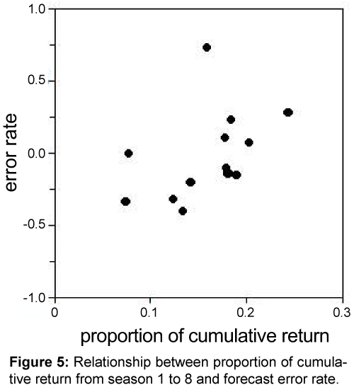
Figure 5: Relationship between proportion of cumulative return from season 1 to 8 and forecast error rate.
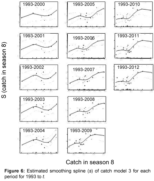
Figure 6: Estimated smoothing spline (s) of catch model 3 for each period for 1993 to t.
I thank Fumihisa Takahashi and Yukihiro Hirabasyashi of the Hokkaido National Fisheries Research Institute, Kei Sasaki of Tohoku National Fisheries Research Institute, and anonymous reviewers, for their useful advice and support.