Forest Research: Open Access
Open Access
ISSN: 2168-9776
ISSN: 2168-9776
Research Article - (2016) Volume 5, Issue 2
The development of effective and accurate models to predict forest growth and products is essential for forest managers and planners. Decision-makers need information on the present yield of the forest for the purpose of monitoring growth. Despite the importance of growth and yield models in the determination of appropriate forest management strategies, no study has been undertaken in IITA’s Forest Reserve. Volume equations for predicting tree volume were developed for tree species in IITA’s Forest Reserve. Complete enumeration of trees larger than 5 cm was carried out in fifteen permanent sample plots of size 20 m × 20 m. The data assessed were diameter at base, diameter at middle, diameter at top, diameter at breast height and total height for 1214 tree species. All trees encountered in each plot were identified with their botanical names. The results revealed that there were 34 important tree species distributed among 23 families in the reserve. The most abundant tree species is Newbouldia laevis while the family with the highest number of species is Moraceae with six species. The number of observations per species ranged from 1 to 255 while the diameter at breast height ranged from 5.00 cm to 201.20 cm and highest percentage of the trees belong to the least diameter class (5-9 cm). The volume equations were fitted for individual species greater than or equal to five and all species combined. The assessment criteria coefficient of determination (R2), Standard error of estimate (SEE) with the validation results (using simple linear regression equation, percentage bias and probability plots of residuals) show that the model of logarithm transformed diameter at base and logarithm transformed total height was of good fit. Very high R2 values, small SEE and percentage biases were obtained. The model was discovered to be very adequate for tree volume estimation in the study area. It is therefore recommended for further use in this ecosystem and in any other forest ecosystem with similar site condition.
<Keywords: Ecosystem, Volume model, Forest inventory, Residual plots, Species
General background
Vanclay [1] defined stand growth models as abstractions of the natural dynamics of a forest stand, which may encompasses growth, mortality and other changes in stand composition and structure. Therefore Forest models can be used as very successful research and management tools. The models designed for research require many complicated and not readily available data, whereas the models designed for management use simpler and more readily accessible data [2]. Growth can be generally defined as the increase in dimensions of an organism or its fraction (forest-forest, stand-individual tree etc.) over time, whereas increment is regarded as the rate of change within a specific period of time [3].
The development of effective and accurate models to predict forest growth and products is essential for forest managers and planners. Growth and yield models, which rely on functions to measurement data from a sample of the forest population of interest, are the tools that have mainly been used to provide decision-support information that meets basic operational needs for evaluating various forest management scenarios [4]. Need for specific information for forest managers and planners are one of the reasons for the increase of the demand for forest models. Growth and yield modeling are very useful tools for managing forest properties either large or small. They are used for operational and strategic planning in nations that own and manage forest lands. Modeling is also good for decision making regarding buying, selling, and trading in forest resources.
Inventories taken at one instant in time provide information on current wood volumes and related statistics [5]. The allometric relationship between tree diameter and total tree height is commonly used to estimate tree volume and thus is a fundamental component of many growth and yield, functional, and forest planning models [6].
IITA Forest Reserve is gradually becoming an endangered ecosystem due to regular poaching activities and exploitation of timber. This ecosystem is an important ecological resource providing many functions and values such as wildlife habitat, water quality protection, biodiversity, timber production and contributes to carbon sequestration. Decision-makers need information on species and biotic type distribution patterns and the effective use of available technology and data at multiple scales of resolution is highly essential. Unfortunately, these information and data is rare [7].
Despite the importance of growth and yield models in the determination of appropriate forest management strategies, relatively few studies have been undertaken on tropical forests. This may be attributed to the existence of multi-species forests with different ages and a wide range of growth habits and stem sizes that pose special challenges to growth modelers. In Africa, only a few growth models have been developed for tree species. The main objective of this research is to develop growth and yield models to predict the growth and yield of a secondary forest in IITA.
The study area
This study was carried out in International Institute of Tropical Agriculture (IITA) forest reserve, it lies on Latitude 07°30’N and longitude 03°55’E at altitude 227 m above sea level in the city of Ibadan, Oyo State. The 350 hectares IITA Forest Reserve has been protected since 1965. The rainfall pattern is bimodal, the mean annual rainfall is about 1301.6 mm most of which falls between May and September. The average daily temperature ranges between 21°C and 23°C while the maximum is between 28°C and 34°C. Mean relative humidity is in the range of 64% to 83% (Figures 1-5).

Figure 1: Map of International Institute of Tropical Agriculture Nigeria.

Figure 2: Relationship between volume and height.

Figure 3: Relationship between volume and Diameter at base.

Figure 4: Relationship between Dbh and Diameter at base.

Figure 5: Relationship between Height and Diameter at breast height.
Data collection
Diameter at breast height (dbh) and total height measurements had been carried out on 15 permanent sample plots (PSP) in the following years: 1975, 2005, 2008 and 2010. Two sets of data on the permanent sample plots (PSP) were used for this study. These are 2008 and 2013 data set. The 2013 data collection was the primary while the 2008 secondary, obtained from the International Institute of Tropical Agriculture (IITA). Complete enumeration of trees larger than 5 cm was carried out in the already demarcated 15 plots of size 20 m × 20 m. Within each plot, the following tree growth variables were measured: Total height, merchantable height, clear bole height, Diameter at breast height (Dbh), Diameter at the base, middle and top, Crown length and diameter.
Measurement of tree growth variables
Crown diameter: Crown measurements were based on the assumption that the vertical projection of a tree crown is circular [8]. Four radii were measured as in Ayhan [9] along four axes at right angle. Along the widest part of the tree crown the tape was held horizontally and extended until each person is vertically under the tip of the longest branch on their side. Measurement was recorded as maximum width. The tape was then turned by 90° and measurement repeated along the thinnest part of the tree crown and recorded as minimum width.
Average crown diameter (Cd) was calculated by summing up the four radii and dividing by 2, thus:
 (1)
(1)
Where;
Cd=average crown diameter
ri=projected crown radii measured on four axes.
Bole diameter: Diameter at breast height (dbh) was measured for all tree individuals by means of a diameter tape. For trees with deformations at 1.3 m, the measurement was made at the sound point on the stem above the abnormality. For buttressed trees, a point of measurement was selected approximately 0.5 m above the convergence of the buttress [10]. Diameter at the top and middle was measured using a spiegel relaskop.
Tree height: Spiegel relaskop was used to measure total height, merchantable height, bole height and crown length.
Data analysis
The data collected from tree measurement was processed into suitable form for statistical analysis. Data processing included basal area estimation, stem volume, crown projection area estimation and tree slenderness estimation.
Basal area estimation: The diameter at breast height (dbh) was used to compute basal area using the given formula
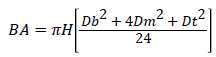 (2)
(2)
Where BA=Basal area (m2), Diameter at breast height (m) and π=3.142
Volume estimation: Volume of each tree was estimated using Newton’s formula as described in Husch et al. [10]
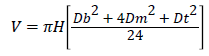 (3)
(3)
Where V=Stem volume (m3), H=height (m), Db=Diameter at the base, Dm=Diameter at the middle, Dt=Diameter at the top and π=3.142
Crown ratio (CR) estimation: Crown ratio was estimated using the formula;
 (4)
(4)
Where THT=Total height and CL=Crown length
Crown projection area estimation: The crown projection area for each tree was estimated using the formula:
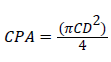 (5)
(5)
Where, CPA=Crown projection area (m2) and CD=Crown diameter (m)
Slenderness coefficient (SLC) estimation: Tree slenderness coefficient was estimated using the formula:
 (6)
(6)
Where, SLC=Tree slenderness coefficient, THT=Total height and dbh=Diameter at breast height
Yield model generation
Volume model developed by Schumacher and Hall [11]; Clutter et al. [12]; Laar and Akca [13] was used for modelling process in this study. However, several forms of this model, using height with the introduction of other variable was considered. This is because height is the major determinant variable if stem volume of tree is considered [11]. In its original form, the model is expressed as:
V=b0Db1Hb2 (7)
Where, V=tree volume (m3); D=diameter at breast height (cm); H=total tree height (m); b0, b1 and b2 are the regression parameters.
Linear, logarithm transformed, quadratic and polynomial forms of regression yield models was adopted. Most equations were directly obtained from the available literature. Some models were modified specifically for the study.
Simple linear regression model
v=b0+b1D (8)
v=b0+b1DH (9)
v=b0+b1CD (10)
Multiple linear regression models
v=b0+b1D+b2H (11)
v=b0+b1 Dm+b2H (12)
v=b0+b1 Dt+b2H (13)
v=b0+b1 Db+b2H (14)
v=b0+b1 D+b2CL (15)
v=b0+b1 BA+b2H (16)
Logarithm transformed models
lnv=b0+b1lnD (17)
lnv=b0+b1lnCD (18)
lnv=b0+b1 lnD2 (19)
lnv=b0+b1 ln DH (20)
lnv=b0+b1 lnD2H (21)
lnv=b0+b1 lnD2+b2lnH (22)
lnv=b0+b1 lnD+b2lnH (23)
lnv=b0+b1 lnDb+b2lnH (24)
lnv=b0+b1 lnDm+b2lnH (25)
lnv=b0+b1 lnDt+b2lnH (26)
lnv=b0+b1 lnBA+b2lnH (27)
lnv=b0+b1 lnD+b2lnCL (28)
lnv=b0+b1 lnD2+b2lnH2 (29)
Quadratic model
v=b0 +b1D2 (30)
v=b0 +b1D2H (31)
v=b0 +b1D2+b2H (32)
v=b0+b1D2+b2H2 (33)
Polynomial models
v=b0+b1D2+b2H+b3D2H (34)
v=b0+b1D+b2H+b3D2+b4H2 (35)
v=b0+b1D+b2D2+b3DH+b4D2H (36)
v=b0+b1D2+b2H2+b3D2H+b4DH2 (37)
Where v=volume (m3), H=Total height (m), ln=natural log, D=Diameter at breast height (Dbh) (m), CL=Crown length (m), CD=Crown diameter (m), Db=Diameter at the base (m), Dm=Diameter at the middle (m), Dt=Diameter at the top (m), b0=regression constant (intercept), b1, b2, b3 and b4=regression coefficients
Volume equations for individual species: In developing volume equations for each of the 34 tree species in this study several model forms were considered and tried for the various species. It was clear that the best model for each species vary in form. The combined variable equation of Spurr [14] and the logarithmic of Schumacher and Hall [11] are classic volume models commonly used, often without question, when developing stem volume equations [15]. The generalized logarithmic model form, which in its original form was the Schumacher-Hall volume model [11], has been used in several studies. The model indicates that tree volume increases proportional to certain powers of D and H. In some previous works [16-18] the D was fixed to the power of 2 while H was fixed to the power of 1 to give the expression;
V=b0+b1D2H+Ɛi (38)
Clutter et al. [12] referred to as the ‘combined variable’ volume function. Model Equation 6 above and the following models were fitted to the data;
SV=b0 +b1D2H (39)
SV=b0 +b1DH (40)
SV=b0 +b1D2+b2H (41)
SV=b0 +b1D2+b2H2 (42)
Where; SV=stem volume, D=Diameter at breast height and H=total height
Assessment of the models
The volume models were assessed with the view of recommending those with good fit for further uses. The following statistical criteria were used:
Significance of regression (F-ratio): This is to test the overall significance of the regression equations. The critical value of F (i.e., Ftabulated) at p<0.05 level of significance was compared with the Fratio (F-calculated). Where the variance ratio (F-calculated) is greater than the critical values (F-tabulated) such equation is therefore significant and can be accepted for prediction.
Coefficient of determination (R2): This is the measure of the proportion of variation in the dependent variable that is explained by the behavior of the independent variable [19]. For the model to be accepted, the R2 value must be high (>50%).
Regression Mean Square Error (RMSE): This is also referred to as the standard deviation or residual of the error variance of the estimate. It measures the spread of data and is a good indicator of precision. The value must be small.
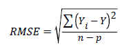 (43)
(43)
Note: Yi=observed value of the dependent variable
Y=predicted value of the dependent variable
n=number of observations
p=number of parameters
Validation of the models
It is highly essential to validate the models selected after assessment before their suitability can be introduced to forest resource management. Validation was done by comparing the models’ output with values observed on the field. This, according to VanHorn [20] is to build an acceptable level of confidence that any inference about the simulated process is correct or valid about the actual process. The validation process also examines the usefulness or validity of the models [21]. The first set (calibrating set) and the second the validation set. The calibrating set is used to construct the models while the validation set is used to test them [22].
All field data were divided into two sets. The first set (calibrating set), comprised growth variables from 971 trees (80%). These were used for generating the models (total volume models) when all species were pooled. The second set (validating set) comprised tree data from 243 trees (20%). These were used for validating the models [23]. For selected species, especially those with few trees, all data were used for calibrating and validating. This was to ensure adequate data to represent different tree growth form and size within a species. Model outputs were individually compared with observed values using the Student t-test for paired means [24] and the simple linear regression equation [25]. In adopting the simple linear regression equation, the observed volume was the dependent variable while the model output was the independent variable.
For models with good fit, there should be no significant difference between the means of the observed and predicted volumes. For the simple linear regression equation, the intercept must approach 0 and the slope approach 1, and the model must be significant (p<0.05 or very high f-ratio value). There must be high correlation between the observed and predicted values, and the coefficient of determination values must also be very high (near 100%) and the standard error of estimates must be small [25-27]. To verify that the residuals are normally distributed and not over or under estimated, residual plots were obtained for all allometric equations by plotting residual values against the independent variate i.e., the predicted volume [28]. While there is many assumptions in the models, the essential multiple leastsquare regression assumptions are that the residuals should have normal distribution with zero mean and constant variance of the residuals.
The student t-test: This was used to test for any significant difference between the actual values or field values and the predicted values (model output) of the various models generated according to Goulding [29,30]
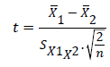 (44)
(44)
and,
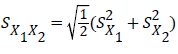 (45)
(45)
Where:
 =Means for predicted and observed data respectively
 =Pooled standard deviation
This is also expected to should show no significant difference in any of the species-size class at 5% level of significance.
Percentage bias estimation: The absolute percentage difference (% bias) was determined by dividing the difference between volumes obtained with Newton’s formula (observed volume) and models output by the same observed volume and multiplied by 100.
% bias=(V0/Vp) × 100 46
Where:
V0=The observe volume
Vp=The predicted volume (models output)
The value must be relatively small for the model to be acceptable for management purpose.
Data summary
The entire data set used for this study consists of 34 species in IITA forest reserve as indicated in Table 1. In terms of their taxonomy, these species belong to 23 different families as indicated in Table 2.
| SNo | Code | Species | Family | Freq. | % Abundance |
|---|---|---|---|---|---|
| 1 | AL | Albizia lebbeck | Fabaceae | 1 | 0.082 |
| 2 | AZ | Albizia zygia | Fabaceae -Mimosoideae | 11 | 0.906 |
| 3 | AC | Alchornea cordifolia | Euphorbiaceae | 2 | 0.165 |
| 4 | ALX | Alchornea laxiflora | Euphorbiaceae | 6 | 0.494 |
| 5 | AA | Antiaris africana | Moraceae | 59 | 4.860 |
| 6 | BN | Barteria nigritiana | Passifloraceae | 1 | 0.082 |
| 7 | BS | Blighia sapida | Sapindaceae | 185 | 15.239 |
| 8 | BB | Bombax buonopozense | Bombacaceae | 2 | 0.165 |
| 9 | CA | Celtis africana | Cannabaceae | 31 | 2.554 |
| 10 | CZ | Celtis zenkeri | Ulmaceae | 3 | 0.247 |
| 11 | CA | Chrysophyllum albidum | Sapotaceae | 87 | 7.166 |
| 12 | CN | Cola nitida | Sterculiaceae | 4 | 0.329 |
| 13 | DG | Dialium guineense | Fabaceae - Caesalpinioideae | 17 | 1.400 |
| 14 | DC | Diospyros crassiflora | Ebenaceae | 1 | 0.082 |
| 15 | FE | Ficus exasperata | Moraceae | 104 | 8.567 |
| 16 | FM | Ficus mucuso | Moraceae | 2 | 0.165 |
| 17 | FU | Funtumia elastica | Apocynaceae | 191 | 15.733 |
| 18 | GA | Gmelina arborea | Verbenaceae | 1 | 0.082 |
| 19 | HF | Holarrhena floribunda | Apocynaceae | 7 | 0.577 |
| 20 | LC | Lecaniodiscus cupanioides | Sapindaceae | 57 | 4.695 |
| 21 | LS | Lonchocarpus sericeus | Fabaceae -Papilionoideae | 1 | 0.082 |
| 22 | ME | Milicia excelsa | Moraceae | 1 | 0.082 |
| 23 | MT | Millettia thonningii | Fabaceae - Papilionoideae | 4 | 0.329 |
| 24 | MI | Mitragyna inermis | Rubiaceae | 3 | 0.247 |
| 25 | MM | Morus mesozygia | Moraceae | 20 | 1.647 |
| 26 | NI | Napoleonaea imperialis | Lecythidaceae | 3 | 0.247 |
| 27 | ND | Nauclea diderrichii | Rubiaceae | 64 | 5.272 |
| 28 | NL | Newbouldia laevis | Bignoniaceae | 255 | 21.005 |
| 29 | PA | Pycnanthus angolensis | Myristicaceae | 13 | 1.071 |
| 30 | SM | Spondias mombin | Anacardiacae | 29 | 2.389 |
| 31 | SG | Syzgium guineense | Myrtaceae | 1 | 0.082 |
| 32 | TM | Trichila monadelpha | Meliaceae | 29 | 2.389 |
| 33 | TA | Trilepisium madagascariense | Moraceae | 16 | 1.318 |
| 34 | TS | Triplochiton scleroxylon | Sterculiaceae | 3 | 0.247 |
| Total | 1214 | 100 |
Table 1: Data distribution according to species.
| S No | Family | No. of Species | No. of Observations | % |
|---|---|---|---|---|
| 1 | Anacardiacae | 1 | 29 | 2.39 |
| 2 | Apocynaceae | 2 | 198 | 16.31 |
| 3 | Bignoniaceae | 1 | 255 | 21.00 |
| 4 | Bombacaceae | 1 | 2 | 0.16 |
| 5 | Cannabaceae | 1 | 31 | 2.55 |
| 6 | Ebenaceae | 1 | 1 | 0.08 |
| 7 | Euphorbiaceae | 2 | 8 | 0.66 |
| 8 | Fabaceae | 1 | 1 | 0.08 |
| 9 | Fabaceae - Caesalpinioideae | 1 | 17 | 1.40 |
| 10 | Fabaceae -Mimosoideae | 1 | 11 | 0.91 |
| 11 | Fabaceae-Papilionoideae | 2 | 5 | 0.41 |
| 12 | Lecythidaceae | 1 | 3 | 0.25 |
| 13 | Meliaceae | 1 | 29 | 2.39 |
| 14 | Moraceae | 6 | 202 | 16.64 |
| 15 | Myristicaceae | 1 | 13 | 1.07 |
| 16 | Myrtaceae | 1 | 1 | 0.08 |
| 17 | Passifloraceae | 1 | 1 | 0.08 |
| 18 | Rubiaceae | 2 | 67 | 5.52 |
| 19 | Sapindaceae | 2 | 242 | 19.93 |
| 20 | Sapotaceae | 1 | 87 | 7.17 |
| 21 | Sterculiaceae | 2 | 7 | 0.58 |
| 22 | Ulmaceae | 1 | 3 | 0.25 |
| 23 | Verbenaceae | 1 | 1 | 0.08 |
| Total | 34 | 1214 | 100 |
Table 2: Data distribution according to family.
A summary of the pooled data for the all species showing number of observations, mean and standard error for each variable is presented in Table 3.
| Variables | Mean | S.E | S.D | C.V | Min. | Max. | Kurtosis | Skewness |
|---|---|---|---|---|---|---|---|---|
| THT | 6.70 | 0.10 | 3.65 | .54 | 1.60 | 31.20 | 4.22 | 1.53 |
| CD | 3.18 | 0.06 | 1.93 | 0.61 | 0.25 | 19.01 | 8.55 | 1.93 |
| DBH | 25.25 | 0.62 | 21.56 | 0.85 | 5.00 | 201.20 | 13.63 | 2.80 |
| DB | 39.23 | 1.03 | 35.99 | 0.92 | 8.00 | 491.00 | 42.30 | 4.91 |
| DM | 13.60 | 0.36 | 12.62 | 0.93 | 2.80 | 124.10 | 16.90 | 3.11 |
| DT | 6.23 | 0.17 | 5.91 | 0.95 | 1.60 | 62.00 | 18.81 | 3.23 |
| CL | 1.91 | 0.03 | 1.13 | 0.59 | 0.20 | 7.00 | 1.52 | 1.17 |
| BA | 0.09 | 0.01 | 0.21 | 2.46 | 0.00 | 3.18 | 94.68 | 8.51 |
| CR | 0.28 | 0.00 | 0.04 | 0.16 | 0.06 | 0.62 | 5.74 | -0.61 |
| SLC | 33.21 | 0.39 | 13.68 | 0.41 | 5.74 | 131.37 | 3.87 | 1.23 |
| CPA | 10.89 | 0.49 | 17.11 | 1.57 | 0.05 | 283.86 | 98.71 | 7.76 |
| VOL | 0.77 | 0.14 | 4.97 | 6.45 | 0.003 | 117.26 | 350.15 | 17.48 |
Table 3: Descriptive statistics for the tree species (2013).THT=Total height (m), CD=Crown diameter (m), DBH=Diameter at breast height (m), DB=Diameter at base (m), DM=Diameter at middle (m), DT=Diameter at top (m), CL=Crown length (m), BA=Basal area (m2), CR=Crown ratio, SLC=Tree slenderness coefficient, CPA=Crown projection area (m2) and VOL=Volume (m3).
The number of observations per species was generally low, with only eleven species having frequencies above 20. Newbouldia laevis (255) has the highest frequency, next to which are Funtumia elastica (191), Blighia sapida (185), Ficus exasperata (104), Chrysophyllum albidum (87), Nauclea diderrichii (64), Antiaris africana (59), Lecaniodiscus cupanioides (57), Celtis africana (31), Spondias mombin (29), and Trichila monadelpha (29).
The family with the highest number of species is Moraceae (6 species). This is followed by Apocynaceae, Euphorbiaceae, Fabaceae- Papilionoideae, Rubiaceae, Sapindaceae and Sterculiaceae with two species each. The family, Fabaceae, is a large family with three subfamilies namely Caesalpiniodeae, Mimosoideae and Papilionoideae. The number of species in these sub-families is 1, 1 and 2, respectively
Growth variables
The result of the descriptive statistics of data collected on growth variables for the species are given in Table 3. The table shows the mean, standard error, standard deviation, co-efficient of variation, minimum, maximum, kurtosis and skewness values of each growth variable.
Diameter and height distribution
Tables 4 and 5 shows the mean, minimum, maximum, standard error and standard deviation values of diameter at breast height in the PSP from 2008 to the year 2013. There has been a decline in the total number of stems in the PSP over the years, which is probably as a result of illegal exploitation hence recruitment of young trees.
| Year | Min. Dbh | Max. Dbh | S.E | S.D | Stem density |
|---|---|---|---|---|---|
| 2008 | 10.00 | 456.00 | 1.31 | 39.12 | 893 |
| 2013 | 5.00 | 201.20 | 0.62 | 21.56 | 1214 |
Table 4: Diameter summary statistics from 2008 to 2013.
| Status | 5-9 | 10-14 | 15-19 | 20-24 | 25-29 | 30-34 | 35-39 | 40-44 | 45-49 | >50 | Stem density |
|---|---|---|---|---|---|---|---|---|---|---|---|
| live trees (2008) | - | 86 | 115 | 106 | 101 | 105 | 63 | 60 | 36 | 221 | 893 |
| live trees (2013) | 285 | 231 | 128 | 99 | 89 | 95 | 69 | 48 | 45 | 125 | 1214 |
Table 5: Life table for the pooled species (2008-2013).
Diameter size class distribution in the PSP year 2013: The distribution of the trees in the Year 2008 and 2013 of the study area into height classes is presented in the Tables 6 and 7 about 94.1% of the measured trees in the Year 2008 fall into the height class (0.1-10 m). This constitutes the largest percentage of the trees in the Year 2008. This was followed by the second height class (10.1-20 m), which had about 3.8%. In the Year 2013 only 0.4% of the trees are in the height class of 20.1-30 m.
| Height (m) | 2008 | 2013 | ||
|---|---|---|---|---|
| Frequency | Percentage | Frequency | Percentage | |
| 0.1-10 | 840 | 94.06 | 1003 | 82.62 |
| 10.1-20 | 34 | 3.81 | 205 | 16.89 |
| 20.1- 30 | 16 | 1.79 | 5 | 0.41 |
| >30 | 3 | 0.34 | 1 | 0.08 |
| Total | 893 | 100 | 1214 | 100 |
Table 6: Distribution of the trees into height classes.
| SLC-class | Frequency | % |
|---|---|---|
| < 70 | 1200 | 98.85 |
| 70-99 | 11 | 0.91 |
| >99 | 3 | 0.25 |
| Total | 1214 | 100 |
Table 7: Slenderness class distribution.
Distribution of growth variables
Slenderness coefficient (SLC) greatly determines the ability of the tree to withstand wind throw. The slenderness coefficient values obtained from the analysis were classified into three categories as suggested by Navratil et al. [31]:
SLC values>99=High slenderness coefficient
70 to 99=Moderate slenderness coefficient
SLC<70=Low slenderness coefficient
Slenderness values usually fall within the range 50-150; slenderness values below 70 are generally an indicator of adequate individual tree stability, 1200 trees have slenderness values of less than 70 which indicate adequate tree stability and 3 trees have high slenderness coefficient. The height of trees in relation to their breast height diameter, their slenderness ratio, seems to be one of the single most important factors determining stem deflection and strength of the tree to resist wind [32]. Trees with a higher slenderness ratio are at risk of firstly being bent sideways by wind then being pulled down by the weight of their crown. Petty and Swain [33] found that slenderness ratio (taper) is probably the most important factor affecting susceptibility to wind breakage with trees of low taper (high slenderness ratio) being much more susceptible to damage. Slenderness values of less than 70 generally produced stability while values of approximately 100 produce instability.
In different studies on the resistance of trees and stands to the action of wind stability of trees is defined by the slenderness factor [34-36]. It is considered as an adequate measure for the determination of stability of trees and their resistance to the action of wind [35,36]. At the same time it needs to be stressed that less regular stands are more stable and thus more resistant to the action of wind than forest monocultures [37].
Crown ratio (CR) is a common indicator of tree vigor [38,39] and is a very useful parameter in forest health assessment used to predict growth and yield of trees and forests. Crown ratio, also as an indirect measure of a tree’s photosynthetic capacity and a measure of stand density, is used as a predictor variable in many existing forest growth and yield models [40,41]. It is also a good indicator of competition and survival potential [42]. It is used as an indicator of wood quality [43], wind firmness [44] and stand density [12].
Table 8 shows that a high proportion of the trees in IITA Forest Reserve have low vigour, this depicts that those with low vigour have small crown length and just one of the trees have high vigour.
| CR-class | Frequency | % |
|---|---|---|
| 0.0-0.3 | 1206 | 99.34 |
| 0.4-0.5 | 7 | 0.58 |
| >0.5 | 1 | 0.08 |
| Total | 1214 | 100 |
Table 8: Crown ratio class distribution.
The size of a tree crown has marked effect on, and is strongly correlated with the growth of the tree and its various parts. It is an indicator of tree vigor. Table 9 shows higher proportions of the trees are in the 0.10-3 size class. The base of live crown varies greatly between and within species, and is usually influenced by growing space, competition, site quality, extent of self-pruning by individual trees, and other factors.
| Crown Diameter class | Freq. | % |
|---|---|---|
| 0.10-3 | 649 | 53.46 |
| 3.10-6 | 482 | 39.70 |
| 6.10-9 | 69 | 5.68 |
| 9.10-12 | 9 | 0.74 |
| 12.10-15 | 3 | 0.25 |
| >15 | 2 | 0.16 |
| Total | 1214 | 100 |
Table 9: Crown diameter class.
Estimates of crown width can also be used to calculate stand canopy closure, which is important for assessing wildlife habitat suitability, fire risk, and understory light conditions for regeneration [45]. Consequently, quantification of crown width attributes is an important component of many forest growth and yield models.
Correlation coefficient of the various growth parameters
There is generally more positive linear relationship between the variables. The highest correlation coefficient value was obtained between diameter at middle and diameter at top (0.99) (Table 10).
| THT | CD | Dbh | Db | Dm | Dt | CL | BA | CR | SLC | CPA | Vol. | |
|---|---|---|---|---|---|---|---|---|---|---|---|---|
| THT | 1 | |||||||||||
| CD | 0.63 | 1 | ||||||||||
| Dbh | 0.83 | 0.72 | 1 | |||||||||
| Db | 0.77 | 0.71 | 0.92 | 1 | ||||||||
| Dm | 0.76 | 0.67 | 0.93 | 0.86 | 1 | |||||||
| Dt | 0.74 | 0.65 | 0.91 | 0.85 | 0.99 | 1 | ||||||
| CL | 0.97 | 0.61 | 0.77 | 0.71 | 0.71 | 0.69 | 1 | |||||
| BA | 0.67 | 0.60 | 0.88 | 0.89 | 0.84 | 0.83 | 0.58 | 1 | ||||
| CR | 0.31 | 0.24 | 0.19 | 0.15 | 0.16 | 0.15 | 0.50 | 0.05 | 1 | |||
| SLC | -0.23 | -0.44 | -0.57 | -0.49 | -0.51 | -0.50 | -0.22 | -0.35 | -0.01 | 1 | ||
| CPA | 0.54 | 0.89 | 0.68 | 0.72 | 0.65 | 0.65 | 0.51 | 0.70 | 0.14 | -0.33 | 1 | |
| Vol | 0.48 | 0.41 | 0.60 | 0.75 | 0.59 | 0.59 | 0.38 | 0.85 | -0.02 | -0.15 | 0.56 | 1 |
Table 10: Correlation matrix for tree growth variables in the study area. THT=Total height (m), CD=Crown diameter (m), Dbh=Diameter at breast height (m), Db=Diameter at base (m), Dm=Diameter at middle (m), Dt=Diameter at top (m), CL=Crown length (m), BA=Basal area (m2), CR=Crown ratio, SLC=Tree slenderness coefficient, CPA=Crown projection area (m2) and Vol=Volume (m3)
The value (0.97) obtained between crown length and total height is also very high and positive. There is a high correlation between some of the variable for example; Dbh and Db (0.92), Dm (0.93), Dt (0.91) and BA (0.88). There is a negative relationship between tree slenderness coefficient and all the other growth variables.
The volume equations
Volume equations for all species combined: The volume equations for all species combined is presented in Table 11a-11e. The results of the simple linear regression volume equations, using dbh, height or crown diameter only as predictor variable, is presented in Table 11a. The model v=b0+b1DH had the highest coefficient of determination (R2) of 0.70; the value of b0 is negative in all the models. However, b1 has a positive value for each of the models. The standard errors are reasonably high.
| Model form | b0 | b1 | R2 | SEE |
|---|---|---|---|---|
| v=b0+b1D | -2.7170 | 13.8040 | 0.36 | 3.9772 |
| v=b0+b1DH | -1.5872 | 1.0060 | 0.70 | 2.7138 |
| v=b0+b1CD | -2.6170 | 1.0640 | 0.17 | 4.5226 |
Table 11a: Simple linear regression volume equations.H=Total height (m), CD=Crown diameter (m), D=Diameter at breast height (m), v=Volume (m3), b0=regression constant (intercept), b1=regression coefficients, R2=Coefficient of Determination and SEE=Standard Error of Estimate.
| Model form | b0 | b1 | b2 | R2 | SEE |
|---|---|---|---|---|---|
| v=b0+b1D+b2H | -2.5429 | 14.5720 | -0.0548 | 0.36 | 3.9772 |
| v=b0+b1 Dm+b2H | -2.7722 | 20.8561 | 0.1053 | 0.35 | 4.0076 |
| v=b0+b1 Dt+b2H | -2.8371 | 42.8348 | 0.1402 | 0.35 | 4.0101 |
| v=b0+b1 Db+b2H | -2.1690 | 12.7459 | -0.3077 | 0.58 | 3.2060 |
| v=b0+b1 D+b2CL | -1.9405 | 17.3746 | -0.8764 | 0.38 | 3.9286 |
| v=b0+b1 BA+b2H | 0.1909 | 21.9217 | -0.1969 | 0.73 | 2.5996 |
Table 11b: Multiple linear regression volume equations.H=Total height (m), Db=Diameter at base (m), Dm=Diameter at middle (m), Dt=Diameter at top (m), D=Diameter at breast height (m), v=Volume (m3), CL=Crown length (m), BA=Basal area (m2), b0=regression constant (intercept), b1 and b2=regression coefficients, R2=Coefficient of Determination and SEE=Standard Error of Estimate .
| Model form | b0 | b1 | b2 | R2 | SEE |
|---|---|---|---|---|---|
| lnv=b0+b1lnD | 1.7569 | 2.4034 | 0.92 | 0.5183 | |
| lnv=b0+b1lnCD | -4.2279 | 2.0508 | 0.48 | 1.3141 | |
| lnv=b0+b1 lnD2 | 1.7552 | 1.2014 | 0.92 | 0.2687 | |
| lnv=b0+b1 ln DH | -2.3880 | 1.4859 | 0.94 | 0.4479 | |
| lnv=b0+b1 lnD2H | -0.7851 | 0.9310 | 0.94 | 0.4285 | |
| lnv=b0+b1 lnD2+b2lnH | -7.2541 | 1.4271 | 2.7607 | 0.82 | 0.7722 |
| lnv=b0+b1 lnD+b2lnH | -1.0679 | 1.7975 | 1.0307 | 0.95 | 0.4278 |
| lnv=b0+b1 lnDb+b2lnH | -2.1228 | 1.8797 | 1.2094 | 0.98 | 0.2740 |
| lnv=b0+b1 lnDm+b2lnH | -1.5735 | 1.4174 | 1.4898 | 0.94 | 0.4625 |
| lnv=b0+b1 lnDt+b2lnH | -1.1840 | 1.2730 | 1.6542 | 0.92 | 0.5042 |
| lnv=b0+b1 lnBA+b2lnH | -0.854 | 0.8982 | 1.0313 | 0.94 | 0.4278 |
| lnv=b0+b1 lnD+b2lnCL | 0.7258 | 1.9689 | 0.6599 | 0.94 | 0.4540 |
| lnv=b0+b1 lnD2+b2lnH2 | -7.2541 | 1.4271 | 1.3803 | 0.82 | 0.7722 |
Table 11c: Logarithm transformed regression volume equations.ln=natural log, H=Total height (m), Db=Diameter at base (m), Dm=Diameter at middle (m), Dt=Diameter at top (m), D=Diameter at breast height (m), v=Volume (m3), CL=Crown length (m), BA=Basal area (m2), b0=regression constant (intercept), b1 and b2=regression coefficients, R2=Coefficient of Determination and SEE=Standard Error of Estimate.
| Model form | b0 | b1 | b2 | R2 | SEE |
|---|---|---|---|---|---|
| v=b0+b1D2 | -0.9339 | 15.4570 | 0.72 | 2.6533 | |
| v=b0+b1D2H | -0.2945 | 0.7607 | 0.93 | 1.3243 | |
| v=b0+b1D2+b2H | 0.1910 | 17.2195 | -0.1969 | 0.73 | 2.5996 |
| v=b0+b1D2+b2H2 | -1.1539 | 14.0425 | 0.0065 | 0.72 | 2.6391 |
Table 11d: Quadratic regression volume equations.H=Total height (m), D=Diameter at breast height (m), v=Volume (m3), b0=regression constant (intercept), b1 and b2=regression coefficients, R2=Coefficient of Determination and SEE=Standard Error of Estimate
| Model form | b0 | b1 | b2 | b3 | b4 | R2 | SEE |
|---|---|---|---|---|---|---|---|
| v=b0+b1D2+b2H+b3D2H | 0.2560 | -11.0001 | 0.0055 | 1.2073 | 0.97 | 0.8955 | |
| v=b0+b1D+b2H+b3D2+b4H2 | 3.8942 | -10.8326 | -0.9213 | 16.22841 | 0.0686 | 0.87 | 1.7793 |
| v=b0+b1D+b2D2+b3DH+b4D2H | -0.7220 | 10.4880 | -18.9775 | -0.5674 | 1.6180 | 0.98 | 0.7734 |
| v=b0+b1D2+b2H2+b3D2H+b4DH2 | 0.3876 | -9.2319 | 0.0064 | 0.9694 | 0.0150 | 0.97 | 0.8874 |
Table 11e: Polynomial regression volume equations.H=Total height (m), D=Diameter at breast height (m), v=Volume (m3), b0=regression constant (intercept), b1, b2, b3 and b4=regression coefficients, R2=Coefficient of Determination and SEE=Standard Error of Estimate
The developed multiple linear regression volume functions (Table 11b), with the exception of the model v=b0+b1BA+b2H, the value of b0 is negative in all the models. However, b1 has a positive value for each of the models. The best multiple linear regression model is v=b0+b1BA +b2H, coefficient of determination (R2) of 0.73.
The results of log-transformed models (Table 11c), with model lnv=b0+b1 lnDb+b2lnH ranked 1st. The criteria adopted for ranking the models was through comparison of coefficient of determination (R2) and standard error of the estimate (SEE) which is one of the standard ways of ranking and validating models as pointed out by Huang et al. [46].
The higher the R2 values the better and the lower the SEE the better. Previous studies such as Akindele [47] have shown that equations with R2 values of 0.86 and 0.96 or higher are considered very good and make good predictors. Low SEE values indicate high level of precision.
The standard error of estimate is a good measure of overall predictive value of regression equations [47]. It is a common measure of goodness of fit in regression models, with low values indicating better fit. In the log-transformed models, the SEE values ranged from 0.2740 to 1.4409.
Table 11d shows the quadratic regression volume equations. The volume function; v=b0 +b1D2H has an R2 value of 0.93, this is probably due to use of the reciprocal of D2H as a weighting factor which appeared to be appropriate for reducing heteroscedasticity. Similar remarks have been made by other researcher including Akindele [47], Cunia [48], Clutter et al. [12] and Philip [49]. Bi and Hamilton [15] explained that this variable represents the volume of a cylinder of diameter D and height H. Stem volume is directly related to the cylindrical volume by the coefficient of this variable that varies with stem form, that is, the solid shape of the stem.
The R2 values ranged between 0.87 and 0.98 for the polynomial regression volume equations generated (Table 11e) for IITA Forest Reserve. All the polynomial regression models developed in this study were discovered to be very adequate for yield estimation in secondary rainforest ecosystem and they are recommended for further use.
Fit statistics: The intercept (b0), slope (b1), coefficient of determination (R2), standard error of estimates (SEE), observed volume, predicted volume and % biases are presented in Table 12a for simple linear models SEE for total volume ranged from 3.8515 to 8.5888. The % biases also ranged from 12.51 to 48.81%. These values were relatively high.
| Model form | b0 | b1 | R2 | SEE | Observed vol. | Predicted vol. | Bias (%) |
|---|---|---|---|---|---|---|---|
| v=b0+b1D | -0.7414 | 2.1198 | 0.56 | 6.8561 | 1.11±0.23 | 31.09 | |
| v=b0+b1DH | -2.6380 | 1.4256 | 0.86 | 3.8515 | 1.62±0.66 | 1.41±0.43 | 12.51 |
| v=b0+b1CD | -0.9416 | 2.8318 | 0.31 | 8.5888 | 0.91±0.13 | 48.81 |
Table 12a: Validation results and % bias of the simple linear models with simple linear regression model.H=Total height (m), CD=Crown diameter (m), D=Diameter at breast height (m), v=Volume (m3), b0=regression constant (intercept), b1=regression coefficients, R2=Coefficient of Determination and SEE=Standard Error of Estimate
Validation results was carried out on the multiple linear models which had a R2 greater than 0.50. There was a high R2 and high standard error of the regression equations as shown in Table 12b. The percentage biases range from 22.87% to 33.45%.
| Model form | b0 | b1 | R2 | SEE | Observed vol. | Predicted vol. | Bias (%) |
|---|---|---|---|---|---|---|---|
| v=b0+b1 Db+b2H | -0.2356 | 1.7186 | 0.82 | 4.3438 | 1.62±0.66 | 1.08±0.35 | 33.45 |
| v=b0+b1 BA+b2H | -0.0412 | 1.3287 | 0.84 | 4.2036 | 1.24±0.46 | 22.87 |
Table 12b: Validation results and % bias of the multiple linear models with simple linear regression model. H=Total height (m), Db=Diameter at base (m), BA=Basal area (m2), b0=regression constant (intercept), b1=regression coefficients, R2=Coefficient of Determination and SEE=Standard Error of Estimate.
The R2 for the log transformed equations ranged from 0.35 to 0.96 for models for predicting total volume and SEE ranged from 0.3597 to 1.4004 (Table 12c). lnv=b0+b1 lnDm+b2lnH had the lowest positive % biases of 2.72%. lnv=b0+b1 lnD2, lnv=b0+b1 lnD2+b2lnH and lnv=b0+b1 lnD2+b2lnH2 had a high negative % biases.
| Model form | b0 | b1 | R2 | SEE | Observed vol. | Predicted vol. | Bias (%) |
|---|---|---|---|---|---|---|---|
| lnv=b0+b1lnD | 0.0518 | 0.9832 | 0.90 | 0.5594 | -1.96 ± 0.11 | -4.41 | |
| lnv=b0+b1lnCD | -0.0137 | 0.9016 | 0.35 | 1.4004 | -2.06 ± 0.07 | -9.95 | |
| lnv=b0+b1 lnD2 | 3.3205 | 0.5794 | 0.90 | 0.5594 | -8.99 ± 0.18 | -378.99 | |
| lnv=b0+b1 ln DH | -0.0006 | 0.9966 | 0.92 | 0.5017 | -1.88 ± 0.11 | -0.23 | |
| lnv=b0+b1 lnD2H | 0.0217 | 0.9946 | 0.92 | 0.4782 | -1.91 ± 0.11 | -1.62 | |
| lnv=b0+b1 lnD2+b2lnH | 1.2580 | 0.7373 | 0.89 | 0.5836 | -4.26 ± 0.14 | -126.88 | |
| lnv=b0+b1 lnD+b2lnH | 0.0178 | 0.9952 | 0.92 | 0.4781 | -1.88± 0.11 | -1.90±0.11 | -1.34 |
| lnv=b0+b1 lnDb+b2lnH | 0.0034 | 0.9867 | 0.96 | 0.3597 | -1.91± 0.11 | -1.54 | |
| lnv=b0+b1 lnDm+b2lnH | -0.0383 | 1.0066 | 0.93 | 0.4358 | -1.83± 0.11 | 2.72 | |
| lnv=b0+b1 lnDt+b2lnH | -0.0382 | 1.0096 | 0.93 | 0.4723 | -1.83 ± 0.11 | 2.99 | |
| lnv=b0+b1 lnBA+b2lnH | 0.0185 | 0.9955 | 0.92 | 0.4781 | -1.90± 0.11 | -1.35 | |
| lnv=b0+b1 lnD+b2lnCL | 0.0469 | 1.0004 | 0.92 | 0.5044 | -1.92± 0.11 | -2.35 | |
| lnv=b0+b1 lnD2+b2lnH2 | 1.2582 | 0.7373 | 0.89 | 0.5836 | -4.25± 0.14 | -126.89 |
Table 12c: Validation results and % bias of the Logarithm transformed regression models with simple linear regression model. ln=natural log, H=Total height (m), Db=Diameter at base (m), Dm=Diameter at middle (m), Dt=Diameter at top (m), D=Diameter at breast height (m), v=Volume (m3), CL=Crown length (m), BA=Basal area (m2), b0=regression constant (intercept), b1=regression coefficients, R2=Coefficient of Determination and SEE=Standard Error of Estimate .
There was a high R2 and high standard error of the regression equations as shown in Table 12d except model v=b0+b1D2H which had a SEE of 2.0346. The percentage biases range from 2.36% to 22.86%.
| Model form | b0 | b1 | R2 | SEE | Observed vol. | Predicted vol. | Bias (%) |
|---|---|---|---|---|---|---|---|
| v=b0+b1D2 | -0.2049 | 1.3664 | 0.83 | 4.2204 | 1.33± 0.44 | 17.58 | |
| v=b0+b1D2H | -0.0969 | 1.0850 | 0.96 | 2.0346 | 1.62± 0.66 | 1.58± 0.60 | 2.36 |
| v=b0+b1D2+b2H | -0.0413 | 1.3287 | 0.84 | 4.2036 | 1.25± 0.46 | 22.86 | |
| v=b0+b1D2+b2H2 | -0.2735 | 1.3711 | 0.84 | 4.1188 | 1.38± 0.44 | 14.79 |
Table 12d: Validation results and % bias of the quadratic models withsimple linear regression model. H=Total height (m), D=Diameter at breast height (m), v=Volume (m3), b0=regression constant (intercept), b1=regression coefficients, R2=Coefficient of Determination and SEE=Standard Error of Estimate.
The R2 for the polynomial models ranged from 0.93 to 0.99 and SEE ranged from 0.9012 to 2.6472 (Table 12e). v=b0+b1D+b2H+b3D2+b4H2 had the only positive % biases of 14.25%. v=b0+b1D2+b2H2+b3D2H +b4DH2 had a high negative % biases of -58.54%.
| Model form | b0 | b1 | R2 | SEE | Observed vol. | Predicted vol. | Bias (%) |
|---|---|---|---|---|---|---|---|
| v=b0+b1D2+b2H+b3D2H | -0.0636 | 1.0139 | 0.99 | 1.1870 | 1.66 ± 0.65 | -2.49 | |
| v=b0+b1D+b2H+b3D2+b4H2 | 0.0332 | 1.1388 | 0.93 | 2.6472 | 1.62 ± 0.66 | 1.39 ± 0.56 | 14.25 |
| v=b0+b1D+b2D2+b3DH+b4D2H | -0.0774 | 0.9987 | 0.99 | 0.9012 | 1.70 ± 0.66 | -4.98 | |
| v=b0+b1D2+b2H2+b3D2H+b4DH2 | -0.6837 | 0.8972 | 0.98 | 1.4023 | 2.56 ± 0.73 | -58.54 |
Table 12e: Validation results and % bias of the polynomial models withsimple linear regression model. H=Total height (m), D=Diameter at breast height (m), v=Volume (m3), b0=regression constant (intercept), b1=regression coefficients, R2=Coefficient of Determination and SEE=Standard Error of Estimate.
The logarithm transformed regression models lnv=b0+b1lnD+b2lnH and lnv=b0+b1lnDb+b2lnH were discovered to have good fit and as a result, they are very adequate for tree volume estimation. This is because of the high coefficient of variation (R2) values and small standard error of estimate. The percentage biases when the output of each model was compared with the observed volume for models lnv=b0+b1lnD+b2lnH is -1.34 and lnv= lnv=b0+b1lnD+b2lnH is -1.54.
The results of the assessment and validation reveal that models lnv=b0+b1lnD+b2lnHand lnv=b0+b1lnD+b2lnH are the best for IITA forest reserves. The fitness and validity of all these models were further confirmed by obtaining the residual plots (i.e. residual values against predicted volume).
A growth and yield model was developed for the growth of a tropical uneven aged secondary forest in IITA forest reserve, Ibadan. This study assessed tree species diversity and also tested the efficacy of linear regression equations for tree volume estimation in IITA forest ecosystem. One thousand two hundred and fourteen trees comprising 34 species distributed among 23 families were involved in model generation.
Stand volume is probably the most important output variable for forest managers, and integrates the effects of height, diameter and density. Volume estimation is critical to forest resource management. Estimation of this parameter is usually confounded by factors such as lack of equipment for measurement of tree height and upper diameter, difficulties in measurement of tree height in tropical forests, the complex architectural structure of tropical forests and the high cost of inventory work. To avoid this problem, models for total volume estimation were developed in this study.
Total volume estimates obtained using logarithm transformed models with height measurements and diameter at base as well as logarithm transformed models with height measurements and diameter at breast height were reasonable.
The prediction of volume in IITA forest reserve required the transformation of dependent and independent variables. Based on validation analyses, logarithm transformed diameter at base and logarithm transformed total height provides a reasonable alternative to other available equations when predicting total volume for IITA forest reserve in Ibadan.
Logarithmic transformation gives better results compared with other untransformed values. This is so because of high variability within and among species in terms of their size and height.
For forest managers, sustainably managing a particular forest tract means determining, in a tangible way, how to use it today to ensure similar benefits, health and productivity in the future. Forest managers must assess and integrate a wide array of sometimes conflicting factors-commercial and non-commercial values, environmental considerations, community needs, and even global impact-to produce sound forest plans.
Forest growth models have become an indispensable tool for forest management. Clearly, models are useful, but they could be more useful. To realize their full utility, models need to become more accurate, and need to become an integral part of the forest management system. Model predictions should be monitored to reveal any discrepancies between predicted and realized outturn. This feedback loop provides the basis for a system of continual improvement both in growth modeling and in forest management.
Growth and yield modeling is an essential prerequisite for evaluating the consequences of a particular management action on the future development of forest ecosystem and has been central theme of Forest Management.
Forests are inherently complex. Models can be useful tools to understand the interactions and dynamic processes occurring in the forest, examine different forest management strategies and their impacts, study the development and evolution of trees and other competing vegetation, graphically visualize the responses of forests to human intervention, or observe ecological and economic interactions of the different components of a forest ecosystem. Forest growth and yield models are used routinely in forest management, and increasingly in other applications (e.g., investigation of impacts of climate change), and many users take their reliability for granted.
Models developed for IITA Forest Reserve can serve as decision support tools that ensure better, sound and sustainable management of the forests. Increasingly, models are becoming more integrated taking advantage of the strengths of each model making them more flexible, robust and user-friendly.
The fitted volume models yielded the statistical outcomes needed for further use. They are sound for volume estimation in this study area and at similar sites. If used outside the study area, some precautions must be taken. The models are recommended for further use. The appropriate use of the developed model may be short-term inventory updating. For long-term projection, the model should be used with caution. Nevertheless, the present model provides a useful tool for forest researchers and managers to predict future stand states.
The cost of forest measurements during forest inventories will be considerably reduced when using volume tables since reliable volume estimates based on two easy measurable variables (height and diameter at base) can be obtained.
Since this forest have no developed growth and yield models, this model has great potential for managers of this forest and should be considered as a useful tool in planning its use and management.