Journal of Thermodynamics & Catalysis
Open Access
ISSN: 2157-7544
ISSN: 2157-7544
Research Article - (2018) Volume 9, Issue 2
Catalysis is usually construed to facilitate equilibrium being attained more easily and quickly, or occasionally less so (anticatalysis), but not to alter the position of equilibrium, i.e., not to alter the equilibrium constant Keq. Indeed, it is sometimes stated that if catalysis could alter Keq, then it could be employed to violate the Second Law of Thermodynamics. Nevertheless, cases wherein catalysis does alter Keq are known. This has been dubbed epicatalysis. A violation of the Second Law via epicatalysis is precluded if it costs at least as much work to restore the catalyst (specifically, the epicatalyst) to its initial state as can be yielded by the alteration of Keq that it can achieve. In most cases of epicatalysis, it does cost at least as much work usually more work to restore the catalyst (specifically, the epicatalyst) to its initial state as can be yielded by the alteration of Keq that it can achieve. Yet recently systems and processes entailing epicatalysis have been investigated for which this may not be true, and hence which may challenge the Second Law. In this paper we investigate a system wherein catalysis alters Keq, yet wherein at least prima facie there seems to be at least in principle zero thermodynamic cost-zero required work for withdrawal and re-insertion of catalysis. Since chemical systems and reactions can be complex, in this paper we instead investigate a simple mechanical-gravitational system that may serve to illustrate the principles more transparently. This system consists a gas particle (e.g., molecule, Brownian particle, etc.) capable of moving within and between two gravitational potential wells separated by a barrier, in a uniform gravitational field.
Keywords: Catalysis; Epicatalysis; Equilibrium constant Keq; Second law of thermodynamics; Work; Negentropy; Free energy
Catalysis is usually construed to facilitate equilibrium being attained more easily and quickly, or occasionally less so (anticatalysis), but not to alter the position of equilibrium, i.e., not to alter the equilibrium constant Keq. Indeed, it is sometimes stated that if catalysis could alter Keq, then it could be employed to violate the Second Law of Thermodynamics. Consider the following cycle, executed isothermally. Insert a catalyst that alters a system’s position of equilibrium or Keq. Then withdraw the catalyst, allowing the system to return (albeit more slowly in the absence of catalysis) to its initial state. The catalyst can then be re-inserted, and the cycle repeated. If, for example, the volume of the system is a function of Keq, then such a cycle could be employed to drive the motion of a piston, thus doing work. It is sometimes stated that such a cycle would violate the Second Law of Thermodynamics, because it represents a heat engine doing work while operating in a cycle despite isothermality [1]. Nevertheless, cases wherein catalysis does alter Keq are known [2-11]. This has been dubbed epicatalysis. A violation of the Second Law via epicatalysis is precluded if it costs at least as much work to restore the catalyst (specifically, the epicatalyst) to its initial state as such a cycle can yield. In most cases of epicatalysis, it does cost at least as much work usually more work to restore the catalyst (specifically, the epicatalyst) to its initial state as such a cycle can yield. Yet recently systems and processes entailing epicatalysis have been investigated for which this may not be true, and hence which may challenge the Second Law [4-11].
Epicatalysis should not be confused with enhanced one-way catalysis. In contrast to standard catalysis, which eases traversal of a potential barrier by the same ratio in both directions, enhanced one-way catalysis eases traversal of a potential barrier only (or at the very least preferentially) in the direction towards equilibrium only (or at the very least preferentially) in the direction towards lower free energy or equivalently towards lower total negentropy. But it does so on either side of equilibrium. And, like standard catalysis but unlike epicatalysis, enhanced one-way catalysis does not work at equilibrium, where free energy or equivalently total negentropy is minimized and thus reaction in either direction is away from equilibrium and hence towards higher free energy or equivalently towards higher total negentropy. Thus, like standard catalysis but unlike epicatalysis-even epicatalysis that does not challenge the Second Law-enhanced one-way catalysis cannot alter Keq, not even with expenditure of at least as much work as such alteration can yield. To re-emphasize, not only does enhanced one-way catalysis not challenge the Second Law, but moreover it cannot alter Keq even in accordance with the Second Law, i.e., even with expenditure of at least as much work as such alteration can yield. Ross discusses and provides references concerning the Second Law in relation to enhanced one-way catalysis in Ross paper [12].
We mention one minor point: Ross considers only cases wherein the Gibbs-free-energy change ΔG is taken to be the criterion for spontaneous change for a system maintained both at constant ambient pressure P and at constant temperature T [12] (Note: We employ P to denote pressure; we will employ P to denote probability). But, to be precise, for ΔG to be the criterion for spontaneous change, this restriction can be somewhat relaxed: (a) ambient pressure P must be maintained strictly constant, but the temperature of a system can varies in intermediate states of a process so long as at the very least it is at the same temperature T in the initial and final states [13]. (b) Since P and T are the natural independent variables for G, under isothermal conditions dG=VdP [13] (For the Helmholtz free-energy change ΔA substitute the volume V of the system for the ambient pressure P and dA=PdV for dG=VdP [13]). But the cases considered by Ross, wherein the Gibbs-free-energy change ΔG is taken to be the criterion for spontaneous change for isobaric, isothermal systems maintained both at constant ambient pressure P and constant temperature T, are the simplest ones in this respect [12]. In this paper we will also consider only a strictly isothermal system, but with our system being sequestered by a uniform gravitational field rather than by constant ambient pressure.
We also mention one clarification [13] it is stated that in an adiabatic process all the energy lost by a system can be converted to work, but that in a nonadiabatic process less than all of the energy lost by a system can be converted to work. But if the entropy of a system undergoing a nonadiabatic process increases, then more than all of the energy lost by this system can be converted to work, because energy extracted from the surroundings can then also contribute to the work output. In some such cases positive work output can be obtained at the expense of the surroundings even if the change in a system’s energy is zero, indeed even if a system also gains energy from the surroundings. Examples: (a) Isothermal expansion of an ideal gas yields work even though the energy change of the ideal gas is zero; heat flow from the surroundings to the ideal gas counterbalancing work done by the ideal gas. (b) Evaporation of liquid water into an unsaturated atmosphere (relative humidity less than 100%) yields work even though liquid water also gains energy in the form of heat from the surroundings in becoming water vapor: evaporation into an unsaturated atmosphere yields work even though it costs heat. According to Bachhuber and Ornes [14-24] in all cases, the total energy of a system plus its surroundings combined is constant: Work is always obtained at the expense of delocalization of energy, i.e., always at the expense of expenditure of negentropy, never at the expense of expenditure of energy. This would not be contravened even if the Second Law of Thermodynamics were violated: Such violation would imply spontaneous localization, but work would still always be obtained at the expense of subsequent delocalization.
In this paper we will investigate a system wherein catalysis alters the equilibrium state, changing the value of the equilibrium constant Keq, yet wherein at least prima facie there seems to be at least in principle zero thermodynamic cost-zero required work-for withdrawal and re-insertion of catalysis. Thus at least prima facie there seems to be for our system at least a Second-Law paradox, and perhaps even a challenge to the Second Law of Thermodynamics. Since chemical systems and reactions can be complex [1-12], in this paper we instead investigate a simple mechanical gravitational system that may serve to illustrate the principles more transparently. For simplicity, we restrict our considerations to the classical domain, wherein both relativistic and quantum effects are negligible.
We briefly review event probability and temporal probability and accept Einstein’s judgment in giving priority to the latter. In the equilibrium constant Keq, and a brief introduction of our system the nature of catalysis (and anticatalysis), and the equilibrium constant Keq, are briefly reviewed, and we briefly introduce our system, consisting a gas particle (e.g., molecule, Brownian particle, etc.,) capable of moving within and between two gravitational potential wells separated by a barrier, in a uniform gravitational field. In Simple mechanical-gravitational system with epicatalysis we discuss our system more thoroughly. The upshot of Simple mechanical-gravitational system with epicatalysis, a consideration of the possible at least prima facie Second-Law paradox posed by our system, that for our system Keq is non-Boltzmann despite thermodynamic equilibrium with an (essentially) infinite heat reservoir and, perhaps more importantly, that in our system Keq can in principle be changed at zero thermodynamic cost, will be discussed in A second-law paradox. The deviation from the Boltzmann distribution and the changes in Keq obtained via Simple mechanical-gravitational system with epicatalysis and A second-law paradox are small, but according to the Second Law of Thermodynamics, because in principle they cost zero, they should be zero. Comparison with existing works, and possible experimental tests and difficulties, we compare our mechanical-gravitational system with epicatalytic systems investigated in previous works [4-11], and briefly discuss possible experimental tests and difficulties pertaining to our system. In robustness of thermodynamics-even in the face of challenges to the second law we discuss the robustness of thermodynamics in general and the Second Law even if some challenges to the Second Law are borne out. We focus particularly on the validity of the Second Law with respect to challenges thereto, and its robustness even if some challenges against it are borne out. Concluding remarks are given in conclusion section. In the Appendix, it is shown that there are realizable ranges of pertinent parameters within which both (a) our gas particle interacts only negligibly with equilibrium blackbody radiation and (b) its translational motion can be treated classically rather than quantum-mechanically.
We distinguish between event probability P and temporal probability Pτ . If a given property Y is discrete, we construe a value y thereof to be a given one from among its discrete values; if a given property Y is continuous, we construe a value y thereof to be a given tiny range  with all ranges being of equal width dy.
We define an event as a sampling of a probability distribution, say of the Boltzmann distribution. Event probability Pε( y) is the fraction of all samplings of its probability distribution-at which a given property Y has a given one value y from among its discrete values if the property Y is discrete, or a value within a given tiny Range if Y is continuous. Temporal probability is the fraction of the time during which a given property Y has a given one value y from among its discrete values if the property Y is discrete, or a value within a given tiny range
  if Y is continuous. For a continuous property Y: event probability density is denoted by temporal probability density is denoted by Pε( y) hence
At thermodynamic equilibrium, and even in nonequilibrium steady state,  are fixed (unchanging with time) for all values of y of any property Y, whether discrete or continuous. In this paper we always assume thermodynamic equilibrium.
Let  be the average time that a given discrete property Y dwells at a given value y overall,
 be the average time that a given discrete property Y dwells at a given value y per individual sampling of this given value y, and
  be the average total time required for a discrete property Y to sample all of its values once. Let
  be the average time that a given continuous property Y dwells within a given tiny range
 overall, be the average time that a given continuous property Y dwells within a given tiny range per individual sampling thereof, and be the average total time required for a continuous property Y to sample all of its ranges once (Important Note: (a) Where used as a subscript, denotes temporal probability as opposed to event probability; where used as a symbol, denotes the time interval that a property Y dwells at a given value. (b) We employ t to denote flight times of our gas particle (e.g., molecule, Brownian particle, etc.). (c) Enclosure within angular brackets denotes an average value:
  if Y is discrete;
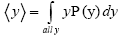 is continuous).
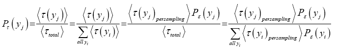
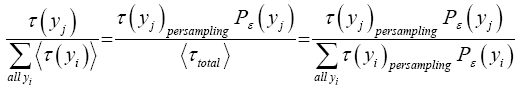
Thus, the temporal probability that one given specified value of a discrete property Y, say yj, obtains is:
 (1)
(1)
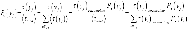
If τ (y)persampling has a fixed (nonfluctuating) value for each and every discrete value y, then the average  collapses to a single value (y) for each and every discrete value y, and Equation (1) simplifies to:
 (2)
(2)
If Y is a continuous property, then the temporal probability that its value lies within a given tiny range, say 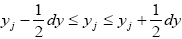 centered at one given specified value of Y, namely yj, is:
 (3)
(3)
If has a fixed (nonfluctuating) value for each and every given tiny range, m  then the average
 collapses to a single value τ(y) for each and every given tiny range
  , and Equation (3) simplifies to:
 (4)
(4)
Thus, temporal probability and event probability for a discrete property Y are related in accordance with Equations (1) and (2). Likewise, temporal probability and probability density on the one hand, and event probability and probability density on the other, for a continuous property Y are related in accordance with Equations (3) and (4). Note that the probabilities in Equations (1-4) are intrinsically normalized to unity.
In this paper we will deal only with continuous or at least effectively continuous properties. An effectively continuous property is or at least may be discrete, but on so fine a scale that for all practical purposes it can be effectively construed as and treated as continuous. Examples include: (a) the translational kinetic energy of a particle that is confined within a fixed finite volume, but with the particle being sufficiently massive, confined within sufficiently macroscopic spatial dimensions, and maintained sufficiently above absolute zero temperature (0K), (b) the molecularity of water measured to the nearest ml, (c) distance and (d) time. In Examples (a) and (b) immediately above discreteness does obtain, but on so fine a scale that for all practical purposes continuity is an excellent approximation. In Examples (c) and (d) immediately above, based on our current imperfect knowledge, discreteness may obtain, but if so only at the Planck scale, a scale even finer; hence for all practical purposes continuity is at the very least an even more excellent approximation.
We accept Einstein’s judgment that the term “probability” should primarily be construed to mean temporal probability [25-28]. We will employ event probabilities in auxiliary roles as necessary, to calculate temporal probabilities, and otherwise. But, in accordance with Einstein’s judgment, in this paper we accept the priority of temporal probability over event probability. Cornelius Lanczos [25] emphasizes that Einstein judged temporal probability to be more fundamental than event probability on a general basis, even though Einstein’s paper cited [25-28] applies the concept primarily to the specific problem of density fluctuations in fluids, focusing especially on a study of critical opalescence. This is confirmed in Einstein’s paper itself, for Einstein discusses the fundamental nature of temporal probability as opposed to event probability in introduction of his paper-wherein he deals with general considerations. Event probability versus temporal probability thereof continues to deal with general considerations. Only in the equilibrium constant Keq, and a brief introduction of our system does Einstein begin to apply these general considerations to the specific problem of density fluctuations in fluids, focusing especially on a study of critical opalescence.
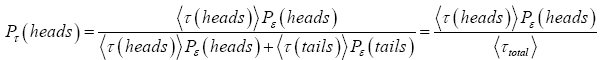
An example may provide clarification concerning event probability versus temporal probability. Perhaps the simplest example that we can consider is the flipping of a single fair coin. The sample space consists of only two states, heads and tails, i.e., the number of possible states is N=2. (We neglect any tiny probability that the coin might land on-edge). The event probability P (heads) of heads or P (tails) of tails-the fraction of all events, i.e., of all samplings of the probability distribution, of all flips of the coin-yielding either heads or tails is Pε (heads)=Pε (tails)=1=N=1=2. But the temporal probability Pτ (heads) of heads or Pτ (tails) of tails-the fraction of the time that the coin lies heads up or tails up-is also 1=2 if and only if the coin is reflipped after an equal elapsed time interval irrespective of whether the result of the immediately preceding flip was heads or tails.But suppose that if the coin lands heads it is reflipped after τ (heads)=1s, whilst if it lands tails it is reflipped after τ (tails)=1y  3.16 107 s. [The dot-equal sign () means “very nearly equal to”]. Of course, the coin is still fair-the event probability of either heads or tails is still Pε (heads)=Pε (tails)=1=2-it is still true that in the long run, letting the number of flips approach infinity, the fraction of flips landing either heads or tails approaches Pε (heads)=Pε (tails)=1=2. (In gambling, which we do not consider in this paper, event probability is usually more pertinent than temporal probability). But the coin will lie tails up (and will be observed to be tails up if anybody looks) almost all of the time: By Equation (2) the temporal probability of heads has only the very small value:
 (5)
(5)
The temporal probability of tails computed either the same way or more simply via
 (6)
(6)
is a near-certainty. If the coin is unfair, then Pτ (heads) ≠ 6 Pτ (tails) ≠ 16 ≠ 2, but Equation (2) remains applicable as per the first line of Equation (5) and the first step of Equation (6). If furthermore, whether the coin is fair or not, τ (heads) and τ (tails) are not constant but instead fluctuate from flip to flip, then we would employ Equation (1) as follows:
 (7)
(7)
with Pτ (tails) computed either the same way or more simply via the first step of Equation (6).
Let a gas particle (e.g., molecule, Brownian particle, etc.) be in either one of two gravitational-potential-energy wells, L or H, or in transit over a barrier from L to H or vice versa via classical thermal motion (For simplicity, we consider barrier transit via classical thermal motion only, and not via quantum-mechanical tunneling). The entire system is in a uniform gravitational field. In both L and H, the gas particle can have a range of gravitational potential energies, but its minimum possible or ground-state gravitational potential energy EH,0 at the bottom of well H equals or exceeds its minimum possible or ground-state gravitational potential energy EL,0 at the bottom of well L. For simplicity and without loss of generality we set EL,0 =0. Thus, our gas particle can have gravitational potential energy (relative to our datum EL,0 =0) EL , EL,0 =0 when it is in well L and EH ≥ EH,0 ≥ EL,0 =0 when it is in well H. A gravitational-potential-energy barrier of height Ebarrier separates L from H. Thus the depth EL of potentialwell L is Ebarrier and that of potential-well H is EH=EbarrierEH, 0. Clearly Ebarrier EH,0 EL,0 =0: the equality in the first sign refers to the special case of a potential-energy step from L to H, that in the second sign to the special case of equal well depths EL =EH=Ebarrier, and both simultaneously to the absence of a barrier, i.e., to Ebarrier =EL,0=EH,0=0. In this paper we do not consider potential steps. The absence of a barrier can be construed as the presence of a barrier of vanishing height. For simplicity we employ a barrier of fixed but negligible width, so that our gas particle is essentially always either in well L or in well H, and essentially never in an intermediate “barrier state” wherein its gravitational potential energy must always equal or exceed Ebarrier .
At thermodynamic equilibrium our gas particle spends a fraction f of its total time in well L and the remaining fraction 1 f of its total time in well H. Thus, at equilibrium it is in well L with temporal probability P(in L)=f and in well H with temporal probability P(in H)=1-f. This is in accordance with Einstein’s judgment that the term “probability” should primarily be construed to mean temporal probability (not event probability): the probability that our gas particle is in a given well is equal to the fraction of its total time that it spends in this given well [25-28]. Equilibrium is most succinctly characterized by the equilibrium constant Keq:
 (8)
(8)
For simplicity we always take both wells to be of the same surface area and the same shape, so if EH;0=EL;0=0 then both wells are identical in every respect-thus if EH,0 =EL,0=0 by symmetry Pτ (in L)=f=Pτ (in H)=1-f=1/2 and hence Keq=1.
Catalysis entails lowering the height Ebarrier of the barrier and/or decreasing its width, thereby rendering transits between wells L and H easier and hence more probable. According to the most commonly-held viewpoint, catalysis renders barrier transits from well L to well H more probable equally, i.e., by the same ratio, as transits from well H to well L. Thus, according to this viewpoint catalysis speeds up the attainment of equilibrium, characterized by Keq, equally, i.e., by the same ratio, from either direction. Hence according to this viewpoint Sienko MJ and Plane RJ [1] catalysis does not, indeed cannot, alter the position of equilibrium-it does not, indeed cannot, alter the value of Keq. Anticatalysis entails raising the height Ebarrier of the barrier and/or increasing its width, thereby rendering transits between wells L and H more difficult and hence less probable. According to the most commonly-held viewpoint, anticatalysis renders barrier transits from well L to well H less probable equally, i.e., by the same ratio, as transits from well H to well L. Thus, according to this viewpoint anticatalysis slows down the attainment of equilibrium, characterized by Keq, equally, i.e., by the same ratio, from either direction. Hence according to this viewpoint anticatalysis does not, indeed cannot, alter the position of equilibrium-it does not, indeed cannot, alter the value of Keq. (For simplicity and in accordance with the last sentence of the first paragraph of the equilibrium constant Keq, and a brief introduction of our system we will focus on altering the height of the barrier rather than on altering its width) [1].
Indeed, according to the most commonly-held viewpoint, if catalysis could alter the position of equilibrium and hence change the value of Keq, then it could be employed to violate the Second Law of Thermodynamics, for example via the following cycle, executed isothermally: Let the equilibrium state E1 of a system in the absence of a catalyst be characterized by the value Keq,1. Insert a catalyst that changes the system’s equilibrium state from E1 to E2, which is characterized by the value Keq,2≠Keq,1. Then withdraw the catalyst and let the system return (albeit more slowly in the absence of the catalyst) to its original equilibrium state E1 characterized by the value Keq,1. The catalyst can then be re-inserted and the cycle repeated. If, for example, E1 and E2 correspond to different volumes occupied by the system, then this cyclic process could be employed to drive the motion of a piston, converting heat into work. If this cyclic process is executed at a single temperature, it would violate the Second Law of Thermodynamics. For the Second Law of Thermodynamics forbids isothermal operation of a cyclic heat engine. An anticatalyst would be employed similarly: Insert an anticatalyst that changes the system’s equilibrium state from E1 to E2, which is characterized by the value Keq,2≠6 Keq,1. Then withdraw the anticatalyst and let the system return (faster in the absence of the anticatalyst) to its original equilibrium state E1 characterized by the value Keq,1. The anti-catalyst can then be re-inserted and the cycle repeated. If again, for example, E1 and E2 correspond to different volumes occupied by the system, then this cyclic process could likewise be employed to drive the motion of a piston, converting heat into work via a cyclic process at a single temperature, in violation of the Second Law of Thermodynamics [1].
In most-but not all-cases catalysts and anticatalysts do not alter the equilibrium state and hence do not alter the value of Keq. But cases wherein they do alter the equilibrium state and hence do change the value of Keq are known [2-11]. In these cases, catalysts and anticatalysts are redubbed epicatalysts and epi-anticatalysts, respectively [4-11]. Nevertheless, contrary to the most commonly-held viewpoint [1] epicatalysis need not challenge the Second Law of Thermodynamics [2-11]. The Second Law is not challenged if it costs at least as much work per cycle to withdraw and re-insert a catalyst or anticatalyst (specifically, an epicatalyst or epi-anticatalyst) and hence to restore it to its initial state as can be yielded via a cyclic process entailing its withdrawal and re-insertion such as described in the immediately preceding paragraph. Thus, according to the Second Law of Thermodynamics a catalyst or anticatalyst (specifically, an epicatalyst or epi-anticatalyst) can itself remain unaltered and hence not require work in order to be restored to its own initial state if and only if it does not alter a system’s equilibrium state and hence does not alter the value of Keq. Yet recently systems processes entailing epicatalysis have been investigated for which this may not be true, and hence which may challenge the Second Law [4-11].
Some system properties
We now investigate a system wherein catalysis alters the equilibrium state, altering the value of Keq, yet wherein at least prima facie there seems to be at least in principle zero thermodynamic cost-zero required work-for withdrawal and re-insertion of catalysis. Thus at least prima facie there seems to be in this case at least a Second-Law paradox, and perhaps even a challenge to the Second Law of Thermodynamics. Since chemical systems and reactions can be complex [1-12], we instead investigate a simple mechanical-gravitational system, briefly already introduced in The equilibrium constant Keq, and a brief introduction of our system, that may serve to illustrate the principles more transparently. The upshot of Simple mechanical-gravitational system with epicatalysis, a consideration of the possible at least prima facie Second-Law paradox posed by our system, that for our system Keq is non-Boltzmann and can in principle be changed at zero thermodynamic cost, will be discussed in a second-law paradox.
Let a single gas particle (e.g., molecule, Brownian particle, etc.,) of mass m be in a uniform gravitational field g, in thermodynamic equilibrium with the ground, which serves as a heat reservoir of (essentially) infinite heat capacity at temperature T. In this paper we always assume thermodynamic equilibrium with a heat reservoir of extremely large-essentially infinite-heat capacity. Such a heat reservoir must typically have an extremely large mass. But a smaller, albeit still decisively macroscopic, mass suffices if the heat reservoir consists of a phase-change material at the temperature of a strongly-first-order phase transition. (Excellent discussions concerning phase transitions are provided in Berry RS [13]. Given thermodynamic equilibrium with such a heat reservoir, the exponential Boltzmann distribution with respect to energy is obeyed exactly [29]. We let the temperature T be low enough (a) to render negligible compared with gas-particle/ground collisions any interaction between the gas particle and equilibrium blackbody radiation corresponding to temperature T, but (b) not so low that the translational motion of our gas particle must be treated quantum-mechanically rather than classically. In the Appendix, it is shown that there are realizable ranges of pertinent parameters within which both (a) and (b) immediately above obtain simultaneously. The discussion is easily generalizable to an N-gas-particle isothermal atmosphere sufficiently rarefied that essentially all gas-particle collisions are with the ground and not with other gas particles. Such a rarefied N-gasparticle isothermal atmosphere is effectively equivalent to N one-gas-particle isothermal atmospheres essentially independent of each other but all interacting with the ground, which serves as their mutual (essentially) infinite heat reservoir at temperature T. A uniform gravitational field is chosen rather than a nonuniform one only for mathematical simplicity: It is the presence of a barrier-in catalysis (lowering the height of the barrier and/or decreasing its width) or anticatalysis (raising its height and/or increasing its width) that, as we will describe, plays the fundamental role in the phenomena considered in this paper.
Thermal flights of our gas particle
Our gas particle of mass m and weight mg samples the event thermal probability, namely Boltzmann, distribution corresponding to temperature T only when it rebounds from the ground [29]. In accordance with the Boltzmann distribution, the event probability of a single gas particle rebounding to a peak altitude within the tiny altitude range 
 (9)
(9)
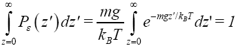
where kB is Boltzmann’s constant. (As noted in Event probability versus temporal probability, we employ P to denote probability and P to denote probability density). This probability is normalized to unity in accordance with
 (10)
(10)
Our single gas particle constitutes a one-molecule isothermal atmosphere whose scale height zscale [corresponding to one e-fold in Pε (z) and Pε (z)] and center-of-mass average altitude
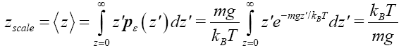 (11)
(11)
Note that Equations (9-11) are valid no matter what altitude z is chosen as datum-level elevation zdatum: zdatum may, but need not, equal zground [29]. Letting z=z-zdatum, Equations (9-11) can be rewritten as [29] respectively.
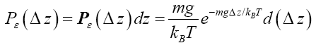 (12)
(12)
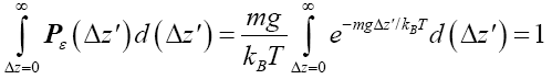 (13)
(13)
 (14)
(14)
The validity of Equations (12-14) given the validity of Equations (9-11) derives from the memoryless property of the exponential probability distribution of Equations (9-14), [30-32]. The exponential distribution is unique in being memoryless [30-32]. Owing to this memory lessness, the probability that the gas particle rebounds to a peak altitude within a tiny altitude range decreases by a factor of e for each increase of z by zscale irrespective of the value of z (and likewise with respect to Δz). We will not need the results of Equations (11) and (14), but they are included for completeness.
Now consider all thermal flights of a gas particle of mass m and weight mg wherein the gas particle attains z directional energy exceeding Ebarrier =mgzbarrier, and hence which can surmount a barrier of height zbarrier above a given ground-level elevation zground. Although we will not need this result as we will not need the results of Equations (11) and (14), it is perhaps interesting to note that, in light of the immediately preceding paragraph, an average barrier-surmounting thermal flight peaks at one scale height over the top of the barrier, i.e., at:
 (15)
(15)
Let us construe two possible geometries of our system. (A) Spherical-surface geometry: Let the surface of our gravitating body, taken as (essentially) spherical and of mass M and radius R for maximum symmetry and simplicity, be divided into a low-elevation (northern) hemisphere that serves as well L and a high-elevation (southern) hemisphere that serves as well H. For simplicity and without loss of generality, and consistently with setting EL;0 =0 in the first paragraph of the equilibrium constant Keq, and a brief introduction of our system, we set ground-level elevation in L at zL,ground=0, at radial distance R from the center of our gravitating body. Let ground elevation in H be zH,ground=N1zscale, i.e., at radial distance R+N1zscale from the center of our gravitating body (N1zscale «R). Also, let there be a barrier at the equator separating the two hemispheres, of height zL,barrier=(N1+N2)zscale « R above ground-level elevation zL,ground=0 in L or equivalently of height zH,barrier=N2zscale «R above ground-level elevation zH,ground=N1zscale in H.
This (essentially) spherical-surface geometry avoids necessitating sufficiently tall walls surrounding our system to (effectively) prevent escape of our gas particle. We let R, and hence also the surface area 2 πR2 of each hemisphere, to be sufficiently large that rebounds from the barrier occur in only a negligible fraction of flights: by the second paragraph of Some system properties, we require that our gas particle thermally rebound (essentially) only from the ground. We take M, R, and m to be large enough, and T to be low enough, to render negligible both the event probability and the temporal probability that our gas particle will thermally rebound from the ground to an altitude exceeding a very small fraction of R, hence justifying our taking g as being constant. (B) Flat-surface geometry: Our system can be construed as occupying only a sufficiently small part of a spherical gravitator of sufficiently large R (such as Earth) that it can be construed to have a flat surface. This necessitates sufficiently tall walls surrounding our system to (effectively) prevent escape of our gas particle. But we take wells L and H, both of the same surface area and the same shape, and separated by the barrier that bisects our system, to be sufficiently large that rebounds from the barrier and from the walls occur in only a negligible fraction of flights: by the second paragraph of Some system properties, we require that our gas particle thermally rebound (essentially) only from the ground. As with the spherical-surface geometry, we take M, R, and m to be large enough, and T to be low enough, to render negligible both the event probability and the temporal probability that our gas particle will thermally rebound from the ground to an altitude exceeding a very small fraction of R, hence justifying our taking g as being constant. For either geometry: (i) M/R can easily still be small enough that the escape velocity from zL,ground=0 is much smaller than the speed of light c, and (ii) T can easily still be high enough that our gas particle’s translational motion can be treated classically. Hence Newtonian theory is adequate, i.e., Einstein’s General Relativity and quantum theory need not be employed. See the Appendix concerning (ii) immediately above. For either geometry, by elementary Newtonian mechanics [33], for a given initial speed of rebound from the ground, maximum horizontal range Rmax (θ) obtains with “launch” at an angle  rad=45°C from the horizontal or vertical, with
 being twice the peak altitude given vertical rebound at the same speed [33]. Hence, even though Equations (9-15) are stated in terms of event probabilities rather than temporal probabilities, letting
Therein, and likewise with respect to the primed dummy variables of integration, gives an indication of the required horizontal extent of the wells L and H if rebounds from the barrier given spherical-surface geometry, and rebounds from the barrier and from the walls given flat-surface geometry, occur in only a negligible fraction of flights. By elementary Newtonian mechanics [33], the time of maximum-horizontal-range flights is proportional only to  , so employing temporal probabilities will not greatly alter said indication. (Of course, we could stipulate that rebounds from the barrier given spherical-surface geometry, and from the barrier and from the walls given flat-surface geometry, are specular rather than thermal, but this is physically unrealistic). Flat-surface geometry, or at least a very close approximation thereto, would almost certainly be employed in any attempt to experimentally test our system: comparison with existing works, and possible experimental tests and difficulties.
Each rebound of our gas particle from the ground in either L or H is a Boltzmann-distribution-sampling event. In accordance with the Boltzmann distribution, the event probability that our gas particle can attain peak altitude exceeding NLpeak zscale above ground-level elevation zL,ground=0 in L is
 (16)
(16)
[For compactness of notation, the subscript “peak” was not used in Equations (9-15) and the associated discussions]. Specifically, the event probability that our gas particle can attain sufficient peak altitude 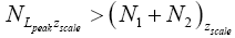 above ground-level elevation zL;ground=0 in L to surmount the barrier is:
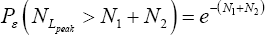 (17)
(17)
Likewise, the event probability that our gas particle can attain peak altitude exceeding NHpeak zscale above ground-level elevation  in H is
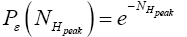 (18)
(18)
(Important Note: NHpeak zscale is taken as the peak altitude attained by a flight originating in H above zH;ground=N1zscale H,ground 1 scale z = N z , not above zL;ground=0). Specifically, the event probability that our gas particle can attain sufficient peak altitude NH peakzscale > N2zscale 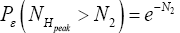 above ground-level elevation zH;ground=N1zscale in H to surmount the barrier is:
Note that Equations (16-19) are compatible with Equations (9-15) if we set NX=z (kBT=mg)=z/zscale, with X being the appropriate subscript for N in the given instance (e.g., X=N1+N2 or X=N2). For brevity in notation, we will sometimes omit the scale height “zscale” when denoting altitudes and denote altitudes dimensionlessly as NX (altitude) zscale =NXz=zscale, i.e., simply as the (dimensionless) number of scale heights NX, with, again, X being the appropriate subscript for N in the given instance (e.g., X=N1+N2 or X=N2).
If our gas particle attains sufficient peak altitude to surmount the barrier, then depending on its location and on its angle of “launch” it may either transit from L to H or from H to L, or land back in its original region, L or H, respectively. But if it does not attain sufficient peak altitude to surmount the barrier, then it must land back in its original region, L or H. Flights of our gas particle entirely within L or entirely within H are dubbed L flights and H flights, respectively. Flights in which our gas particle does not attain sufficient peak altitude to surmount the barrier and hence must remain in its original region, L or H, are dubbed mandatory L flights and mandatory H flights, respectively. Flights during which our gas particle does attain sufficient peak altitude to surmount the barrier and hence can transit from its original region, L or H, to H or L, respectively, yet still remains in its original region, L or H, are dubbed nonmandatory L flights and nonmandatory H flights, respectively. Flights from L to H and from H to L are dubbed L → H transit flights and H → L transit flights, or for short L → H transits and H → L transits, respectively.
Probabilities of our gas particle being in well l, in well h, or in transit
Let Pε (in L) be the event probability that our gas particle is in L and Pε (in H) be the event probability that it is in H.
 be the conditional event probability [34] that our gas particle transits to H given that it is initially in L AND that it attains sufficient peak altitude
  to surmount the barrier. (The abbreviated notation with “in L AND” deleted is expedient because altitude given in terms of NL implies that our gas particle is in L). Then the overall event probability that, on any given flight, our gas particle if initially in L transits to H is [34].
 (20)
(20)
Likewise, let  be the conditional event probability that our gas particle transits to L given that it is initially in H AND that it attains sufficient peak altitude
  to surmount the barrier. (The abbreviated notation with “in H AND” deleted is expedient because altitude given in terms of NH implies that our gas particle is in H). Then the overall event probability that, on any given flight, our gas particle if initially in H transits to L is [34].
 (21)
(21)
Perhaps we should clarify that Pε [(L → H)|(in L)] > Pε (L → H) and likewise that Pε [(H → L)|(in H)]>Pε (H → L). For
 (22)
(22)
Likewise  (23)
(23)
The second steps in the second lines of Equations (22) and (23) are justified because 
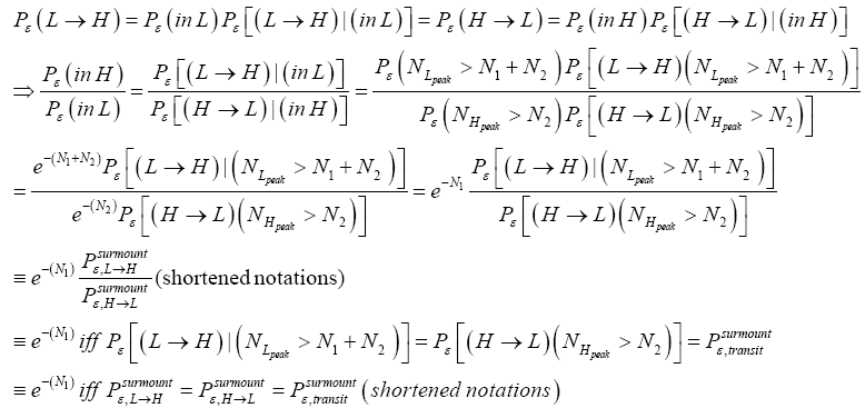
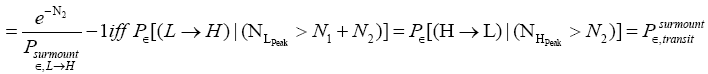
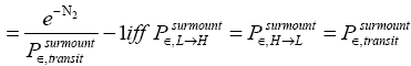
Detailed balance requires that given thermodynamic equilibrium AND given that our gas particle has attained sufficient altitude to surmount the barrier, L → H and H → L transits must be equiprobable. Applying equations (20-23), this requirement is met if and only if [abbreviated as if in the last two lines of Equations (24,27,28)].
 (24)
(24)
(Important Note: The shortened notations  for
for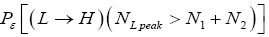 and
and  for
for 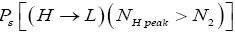 introduced in the fourth line of Equation (24) hopefully are self-explanatory, but just in case:
 the conditional event probability [34] of an L → H transit given that our gas particle has attained sufficient altitude in L to surmount the barrier, and
 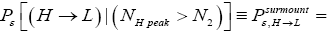 the conditional event probability of an H → L transit given that our gas particle has attained sufficient altitude in H to surmount the barrier). To re-emphasize, as per the last four lines of Equation (24), we must have:

 (25)
(25)
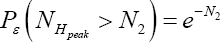
if detailed balance is to yield | P (inH ) / P (in L) = e−N1 ε ε as required by the Second Law of Thermodynamics-specifically by the Boltzmann distributiongiven thermodynamic equilibrium with a heat reservoir of (essentially) infinite heat capacity. This can obtain if and only if, given thermodynamic equilibrium AND given that our gas particle has attained sufficient altitude to surmount the barrier,  is equal in both directions. Note that the derivation of detailed balance, as summarized in this paragraph, is in terms of event probabilities rather than temporal probabilities. Likewise, the equiprobability of in both directions given thermodynamic equilibrium and given that our gas particle has attained sufficient altitude to clear the barrier is event equiprobability rather than temporal equiprobability. Ideally, detailed balance and said equiprobability should be expressed in terms of temporal, not event, probabilities [25-28,35,36]. Yet the consideration of detailed balance and said equiprobability given here in terms of event probabilities is sufficient, indeed what will be required, for our subsequent derivations in terms of temporal probabilities. The event equiprobability represented by Equations (24) and (25), in particular by the last two lines of Equation (24) and by Equation (25), will be employed to help derive temporal probabilities that we will later require, as will be clarified in Average number of flights per well occupation and A second-law paradox (The shortened notations
  for
for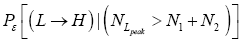 and
and 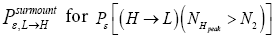 will render some subsequent equations less cumbersome).
Average number of flights per well occupation
Let an event have an event probability P of occurring and an event probability 1-Pε of not occurring at any one given trial or attempt, i.e., at any one given sampling of its event-probability distribution. If, as is true in all instances that we consider, these samplings of its event-probability distribution are Bernoulli trials [37] and hence statistically independent, then the probability of exactly N consecutive non-occurrences is directly proportional to (1→P)N and is equal to 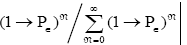 Obviously N can be any non-negative integer. Thus, the average number of econsecutive non-occurrences before the first occurrence is [38].
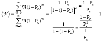 (26)
(26)
The denominator  is a normalizing factor required because the probability distribution per N=0 se is not normalized to unity, i.e.,
 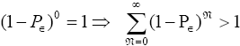 . But the probability distribution
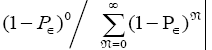 is normalized to unity.
Thus, applying Equations (20) and (26), if our gas particle is in L it will on the average undergo
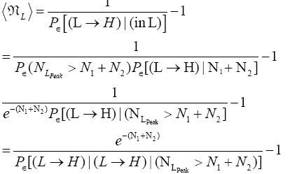 (27)
(27)

 (shortened notation)
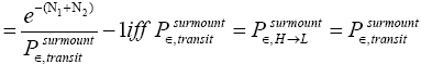
L flights before transiting to H. Likewise, applying Equations (21) and (26), if our gas particle is in H it will on the average undergo
 (28)
(28)
 (shortened notation)
H flights before transiting to L (As mentioned in the last sentence of Probabilities of our gas particle being in well L, in well H, or in transit, the shortened notations for
for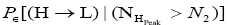 and
and render some equations subsequent thereto less cumbersome).
Time spent in flights, in transits, and in wells
by elementary Newtonian mechanics [33], a round-trip (up and back down) L flight that peaks at altitude NLpeakzscale requires time
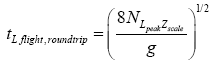 (29)
(29)
And the one-way halves (up or back down) of an L flight that peaks at altitude NHpeakzscale each requires half this time [33]:
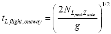 (30)
(30)
Likewise, by elementary Newtonian mechanics [33], a round-trip (up and back down) H flight that peaks at altitude NH peakzscale NHpeakzscale requires time
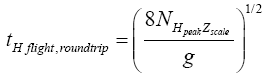 (31)
(31)
And the one-way halves (up or back down) of an H flight that peaks at altitude NHpeakzscale each requires half this time [33].
Even though this is a well-known result of elementary Newtonian mechanics, it is important to emphasize that the time required for a roundtrip (up and back down) flight and for the one-way halves (up or back down) thereof depends only on the flight’s peak altitude and not at all on its horizontal range. For the vertical and horizontal components of motion are independent: Vertical motion during a flight proceeds independently of any horizontal motion, as if the horizontal motion didn’t even exist [33]. In accordance with Einstein’s judgment [25-28], we accept the priority of temporal probability over event probability. When all is said and done, we will ultimately require temporal probabilities for our derivation of Keq. Temporal probabilities relate to time; hence it is the times of flights that are of primary interest to us (Of course, only for flights short compared to the radius R of our (essentially) spherical gravitator, for which g can be taken as constant, does the flight time depend only on the peak altitude. But such flights are the only ones of interest to us).
The event probability of a flight peaking at 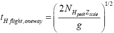 (32) scale heights above ground elevation is
  and in accordance with elementary Newtonian mechanics [33] by Equations (29-32) the time required for such a flight in a uniform gravitational field is proportional to
Thus, evaluations of average time durations-and hence of temporal probabilities-of L flights and H flights entail integrals of the form 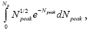 where for example NX=N1+N2 for L flights whose peak altitude fails to exceed the barrier height, NX=N2 for H flights whose peak altitude fails to exceed the barrier height, and NX=∞ for flights peaking at arbitrary altitude. According to the Online Integral Calculator at Wolfram Math World [39]:
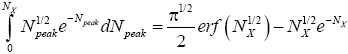 (33)
(33)
where  is the error function [40] of
  This integral can be evaluated as a rapidly-converging power series in each of the two limiting cases
 We will find it sufficiently accurate to retain only the first term in NX of these power series [39]:
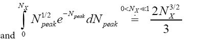 (34)
(34)
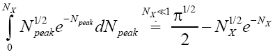
The right-hand side of Equation (35) should be obvious on inspection of Equation (33), because 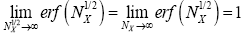 (35) [39,40].
In the extreme case NX=0, this integral obviously vanishes: 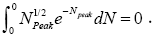 In the opposite extreme case NX=∞ [39],
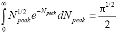
Thus, the value of this integral increases monotonically from 
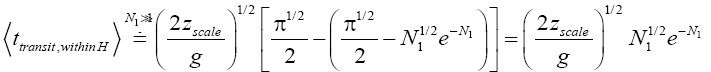
Let 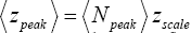 be the average peak altitude of any given category of flights: mandatory L flights, nonmandatory L flights, mandatory H flights, nonmandatory H flights, complete L → H or H → L transits, or the parts of transits within L or within H. For all flights except mandatory L flights and mandatory H flights, NX=∞. Applying Equations (29), (31), and (36), for nonmandatory L flights and for nonmandatory H flights [33,39,40],
 (37)
(37)
Applying Equations (29) and (33-35) [33,39,40], for mandatory L flights:
 (38)
(38)
 (39)
(39)
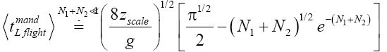 (40)
(40)
Likewise, applying Equations (31) and (33-35) [33,39,40], for mandatory H flights:
 (41)
(41)
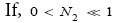
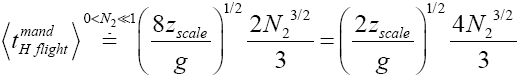 (42)
(42)
 (43)
(43)
Apply Equations (16,17,36-40). Recall that for mandatory L flights NL peak cannot exceed N1+N2.
Also recognize that a fraction 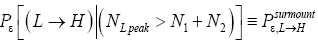 of L flights attaining
 transit to H and hence are L → H transits, and thus that the remaining fraction
  of these flights are nonmandatory L flights (flights that attain
 yet do not transit to H but remain in L). Let
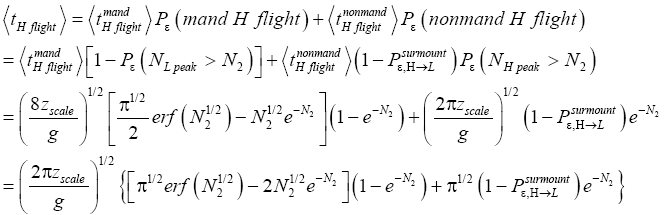
 be the average time required per L flight, averaging over all L flights, mandatory and nonmandatory. Thus:
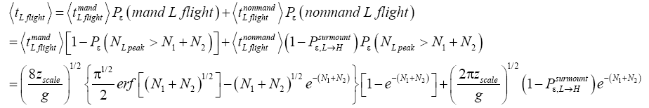 (44)
(44)
 (45)
(45)
 (46)
(46)
Likewise, apply Equations (18,19,36,37,41-43). Recall that for mandatory H flights NH peak cannot exceed N2. Also recognize that a fraction  of H flights attaining NH peak>N2 transit to L and hence are H → L transits, and thus that the remaining fraction
  of these flights are nonmandatory H flights (flights that attain NH peak>N2 yet do not transit to L but remain in H). Let
  be the average time required per H flight, averaging over all H flights, mandatory and nonmandatory. Thus:
 (47)
(47)
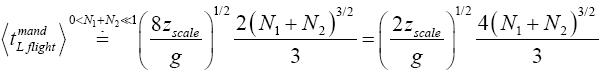
If  employing the very close approximation
 (48)
(48)
If 
 (49)
(49)
Applying Equations (30) and (36), for the parts of both L → H and H → L transits within L, for which the barrier height is (N1+N2) zscale [33,39,40],
 (50)
(50)
Applying Equations (32-36), for the parts of both L → H and H → L transits within H, for which the barrier height is N2zscale, i.e., N1zscale less than for the parts of transits within L [33,39,40].

 (51)
(51)
If,  employing the very close approximation
  valid given
 (52)
(52)
If 
 (53)
(53)
Note the difference between the relations for  This difference obtains because, although as per Equations (30) and (32) and the paragraph containing Equations (33-36) the upper limits of integration are the same, namely NX=∞, for the parts of both L → H and H → L transits within L and the parts of both L → H and H → L transits within H, the lower limits of integration are different, namely 0 for the parts of both L → H and H → L transits within L and N1 for the parts of both L → H and H → L transits within H. This of course, obtains because ground elevation is 0 in L but 1 scale N z in H. Thus, we account for the vertical distance that must be traversed during the parts of both L → H and H → L transits within H being smaller by 1 scale N z than the vertical distance that must be traversed during the parts of both L → H and H →L transits within L.
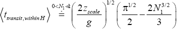
An average visit of our gas particle to L consists of the second part of an H → L transit that by Equation (30) is counted as being within L, followed by  (mandatory and nonmandatory) L flights, followed by the first part of an L → H transit that by Equation (30) is counted as being within L. We denote the average total time required for the a for mentioned parts of two transits that are counted as being within L by 2
  . Hence, applying Equations (16,17,27,29,30,33-40,44-46,50), the average time that our gas particle spends per visit to L is:

 (54)
(54)
If 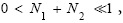 employing the very close approximation ex=1+x valid given
 (55)
(55)
If 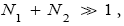
 (56)
(56)
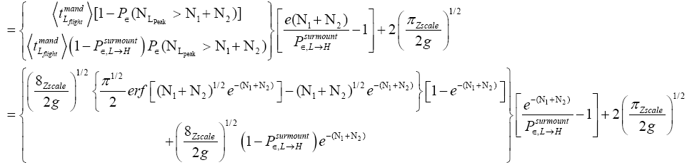
An average visit of our gas particle to H consists of the second part of an L → H transit that by Equation (32) is counted as being within H, followed by  (mandatory and nonmandatory) H flights, followed by the first part of an H → L transit that by Equation (32) is counted as being within H. We denote the average total time required for the aforementioned parts of two transits that are counted as being within H by 2
  . Hence, applying Equations (18,19,28,31-37,41-43,47-49,51-53), the average time that our gas particle spends per visit to H is:
 (57)
(57)
Valid given 
 (58)
(58)
If 
 (59)
(59)
Our result for Keq
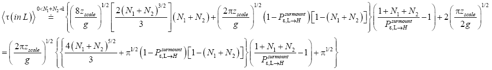
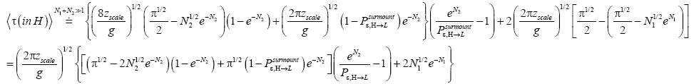
Applying the last two lines of Equation (24), Equation (25), the last two lines of Equations (27 and 28), and 1=2 Equations (54-59), and omitting the prefactor  that is common to both
 and
and  as per the last lines of Equations (54-59), we have
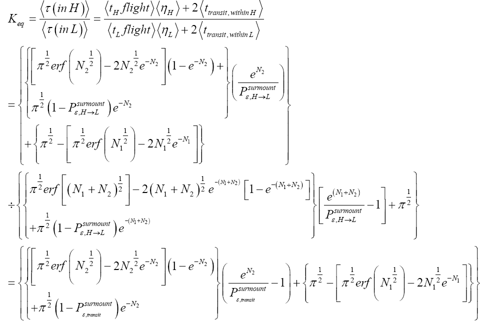
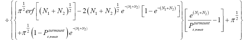 (60)
(60)
If  employing the very close approximation e=1+x valid given
If N1+N2 « 1,
Note that: (a) The consideration of detailed balance in terms of event probabilities in accordance with Equations (24) and (25) and the associated discussions [especially the application of the last two lines of Equation (24) and Equation (25)], and (b) the consideration of  and
and in terms of event probabilities in accordance with Equations (26-28) and the associated discussions [especially the application of the last two lines of Equations (27) and (28)], is sufficient, indeed what is required, for our derivation of Keq as a ratio of temporal probabilities in Equation (60), and hence also in the limiting cases thereof represented by Equations (61) and (62). It is employed in Equations (60-62) only at the last steps [at the last equal (=) signs] thereof. Thus, detailed balance in terms of event probabilities, and and in terms of event probabilities, help us to derive Keq as a ratio of temporal probabilities in Equations (60-62).
Is Keq non-boltzmann and changeable for free? a second-law paradox?
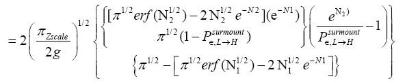
Unfortunately, our result for Keq in Equation (60), and even in the limiting cases thereof represented by Equations (61) and (62), is somewhat cumbersome, and there seems to be no obvious way to simplify it further. But our result for Keq in Equation (60), and hence also in the limiting cases thereof represented by Equations (61) and (62), does not equal the Boltzmann factor e-N1, as the Second Law of Thermodynamics would seem to require given thermodynamic equilibrium with an (essentially) infinite heat reservoir: It is slightly smaller than e-N1 and hence slightly different from e-N1. Our result for Keq in Equation (60), and hence also in the limiting cases thereof represented by Equations (61) and (62), is only slightly smaller than, and hence only slightly different from, the Boltzmann factor e-N1 that the Second Law of Thermodynamics would seem to require given thermodynamic equilibrium with an (essentially) infinite heat reservoir. But while this difference from the Boltzmann factor e-N1 is small, we seek only to show that it is not zero, i.e., that it exists at all.
Our result for Keq as per Equation (60), and hence also as per the limiting cases thereof represented by Equations (61) and (62), being slightly smaller than e-N1 owes to well H being shallower than well L. {In accordance with the last two lines of Equation (24), with Equation (25), and with the last two lines of Equations (27,28), at the last steps [at the last equal (=) signs] of Equations (60-62) we take:

There are three well-H/well-L deficits and corresponding ratios: (a) By Equations (38-43) if N1 > 0 on average mandatory H flights require less time than mandatory L flights. Since by Equation (37) on average nonmandatory L flights and nonmandatory H flights require equal time, considering all flights, mandatory and nonmandatory, if N1 > 0 the first ratio in the last term of first line of Equation (60), namely  is smaller than unity. (b) Owing to the last term (1) in Equations (26-28), especially in the last two lines of Equations (27) and (28) where we take
 if N1 > 0 the second ratio in the last term of first line of Equation (60), namely
  is smaller than e N1, and hence the average number of H flights before transit to L is less than e-N1 times the average number of L flights before transit to H. (c) By Equations (50-53) if N1 > 0 on average the parts of L → H and L → H transits in H require less time than the parts thereof in L. Hence if N1 > 0 the third ratio in the last term of first line of Equation (60), namely
Furthermore, and perhaps more importantly, not only is Keq slightly smaller than, and hence slightly different from, the Boltzmann factor e-N1, but how much smaller and hence how much different can be changed by altering the barrier height. For, the magnitudes of the three well-H/well-L deficits and corresponding ratios (a), (b), and (c) elucidated in the immediately preceding paragraph are functionally dependent on the barrier height. Moreover at least prima facie there seems to be at least in principle zero thermodynamic cost-zero work required-for raising or lowering the barrier and thereby altering Keq. If the barrier is raised, another weight can be lowered in compensation; if the barrier is lowered, another weight can be raised in compensation. Also, PdV work done against the equilibrium blackbody radiation corresponding to temperature T, and against our extremely rarefied isothermal atmosphere at temperature T, when the barrier is raised can in principle be recovered when it is lowered. Thus, at least prima facie, it seems that in principle the network required to effect a small isothermal change Keq in Keq in our system is zero, rather than  as required by the Second Law of Thermodynamics.
Note that if ground-level elevations are equal in L and H, i.e., if zH;ground=zL;ground ⇔ N1=0 and hence zbarrier;H=zbarrier;L=N2zscale, and if in accordance with the last two lines of Equation (24), with Equation (25), and with the last two lines of Equations (27) and (28), we take  as we do in the last steps [at the last equal (=) signs] of Equations (60)-(62), then, in accordance with the paragraph containing Equation (8) (especially the last sentence thereof), Equation (60), and hence also the limiting case thereof represented by Equation (61), yield Keq=1, as the Second Law of Thermodynamics requires given thermodynamic equilibrium with an (essentially) infinite heat reservoir. Indeed ground-level elevations being equal in L and H is the only circumstance wherein our system does not pose a Second-Law paradox-the only circumstance wherein the well-H/well-L deficits (a), (b), and (c) expounded in the two immediately preceding paragraphs do not obtain, i.e., vanish, and hence the only circumstance wherein the corresponding ratios (a), (b), and (c) expounded therein all individually equal unity. Thus to emphasize not only do Equations (60) and (61) then yield Keq=1, but furthermore all corresponding individual terms in
  and
and i.e., in the numerator and denominator (too lengthy to be put in the usual form of numerator/denominator, so put in the form numerator denominator) in Equations (60) and (61) are equal. Equivalently, not only do Equations (60) and (61) then yield Keq=1, but furthermore each of the three ratios (a), (b), and (c), i.e.,
  and
and  respectively, in the last term of first line of Equation (60) then individually equals unity (Equation (62), which considers the limiting case N1 ≫ 1, obviously is inapplicable in the opposite limiting case 0
Ground elevations in L and H must be unequal, i.e., we must have zH;ground>zL;ground=0 ⇔ N1 > 0 and hence zbarrier;L=(N1+N2)zscale > zbarrier;H=N2zscale, if processes are to require unequal times in L and H. Moreover, the overall degree of difference of the inequality  from the Boltzmann factor e-N1 is a function of the barrier height and hence can be changed, at least prima facie for free as per this The upshot: is Keq non-boltzmann and can Keq be changed for free. This is in keeping with Einstein’s judgment [25-28] concerning the primacy of temporal probability over event probability.
Note that all the three well-H/well-L deficits and the respective corresponding ratios (a) 
 , respectively, in the last term of first line of Equation (60) and expounded in the second through fifth paragraphs of A second-law paradox are temporal-probability based.
Both ratio  are expressed explicitly in terms of time. Ratio (b) hNHi=hNLi is expressed implicitly in terms of time. Ratio (a)
 is the ratio of the average time
  per H flight to the average time
  per L flight, not counting transit flights.
 is the ratio of the number of H flights per visit of our gas particle to H to the number of L flights per visit of our gas particle to L, not counting transit flights. Thus the product [ratio (a)
  equals the ratio of the average time per visit to H to the average time per visit to L, not counting transit times.
While we have employed both statistical thermodynamics and kinetic theory, it is primarily the kinetic-theory aspects that, at least prima facie and at least in principle, seem to facilitate Keq being non-Boltzmann, and especially to facilitate Keq being alterable for free, at zero thermodynamic cost, without work. Since kinetic theory entails the times required by processes and hence ultimately  this also is in keeping with Einstein’s judgment [25-28] concerning the primacy of temporal probability over event probability. (Recall especially the five immediately preceding paragraphs).
We again note that catalysis entails lowering the height of the barrier and/or decreasing its width, and anticatalysis entails raising its height and/ or increasing its width-but also that, for simplicity and in accordance with the last sentence of the first paragraph of The equilibrium constant Keq, and a brief introduction of our system, we focused on altering the height of the barrier rather than on altering its width. Nevertheless, we should also note that at least prima facie there also seems to be at least in principle zero thermodynamic cost-zero net required work-for widening or narrowing the barrier. Unlike raising or lowering the barrier, widening or narrowing it entails no gravitational-potential-energy changes. But PdV work done against the equilibrium blackbody radiation corresponding to temperature T, and against our extremely rarefied isothermal atmosphere at temperature T, when the barrier is widened can in principle be recovered when it is narrowed.
Comparing this present work with existing works pertaining to epicatalysis and the Second Law of Thermodynamics, the simple mechanicalgravitational system considered in this paper, even if it does pose a Second-Law paradox, or perhaps even a challenge to the Second Law, seems much less amenable to practicable utilization than the epicatalytic systems investigated in existing works. It would probably be considerably more difficult even to test our system experimentally than the epicatalytic systems investigated in existing works, which have already undergone experimental tests. But because of the simplicity in principle of our mechanical-gravitational system in comparison to the chemical systems investigated in existing works, hopefully we have been able to investigate it more thoroughly in principle, from a theoretical rather than experimental perspective [4-11].
Even so, perhaps experimental tests of our mechanical-gravitational system might be possible. Flat-surface geometry, or at least a very close approximation thereto, almost certainly would be more easily employable than sphericalsurface geometry in any experimental tests of our system. (Recall the third paragraph of Average number of flights per well occupation for brief discussions of these two geometries). Also, experimental tests of our system might be less problematic if, instead of a single gas particle, there is employed an atmosphere of many, but sufficiently rarefied that essentially all gas-particle collisions are with the ground rather than with other gas particles. (Recall the second paragraph of some system properties). This would facilitate experimental tests in much shorter times than would be required to ascertain the long-time average behavior of a single gas particle. Long times are required to ascertain the average behaviour of a single-particle system (or even a few-particle system), even if, as the system discussed in this paper, it is in thermodynamic equilibrium with an (essentially) infinite heat reservoir. Much shorter times are required to ascertain the average behavior of a many-particle system, whether it is in thermodynamic equilibrium with an (essentially) infinite heat reservoir. Brownian particles rather than molecules might be employed, so that this rarefied atmosphere has a conveniently small-scale height in Earth’s gravitational field. Owing to their larger masses, Brownian particles have much larger average thermal momenta than molecules (albeit the same average thermal kinetic energies), so perhaps their impacts with the ground could be more easily detected. Also, owing to their larger masses and sizes, Brownian particles could likely be observed with light sufficiently weak that their thermal momenta are only negligibly affected. Losses owing to irreversible effects such as friction, information-processing costs [41-44] (originally attributed to the cost of observation [41,42] but currently attributed to the cost of erasure from memory [43,44]), etc., that obtain in practice would need to be subtracted to determine whether or not our system poses a Second-Law paradox, or perhaps even a challenge to the Second Law, in principle.
A centrifugal field, essentially uniform over small radial displacements jrj r, might be employed. (The strong inequality jrj r implies that to within a very close approximation flat-surface geometry obtains for our system). But this entails additional experimental difficulties. For example, the free-energy/negentropy costs of initiating rotation and then maintaining it against friction in practice would need to be subtracted to ascertain whether or not our system poses a Second-Law paradox, or perhaps even a challenge to the Second Law, in principle. And, of course, Earth’s gravitational field, uniform over the small sizes of experimental apparatuses, is always superposed on the centrifugal field.
Alternatively, perhaps electrically-charged gas particles might be employed, in a uniform electrostatic field, as, say, between parallel capacitor plates. The gas particles might be Brownian-size ones such as those employed in determining the elementary charge per electron [45]. But this also entails additional experimental difficulties. Losses owing to the free-energy/negentropy costs of setting up the electric field and charging the gas particles that obtain in practice would need to be subtracted to ascertain whether or not our system poses a Second-Law paradox, or perhaps even a challenge to the Second Law, in principle. If electrons, say from the inner surfaces of the capacitor plates, were employed as gas particles, high temperatures probably would be required, because the work functions of even the alkali metals are much greater than kBT at room temperature [45- 47]. The free-energy/negentropy costs of generating and maintaining the required temperature in practice would need to be subtracted to ascertain whether or not our system poses a Second-Law paradox, or perhaps even a challenge to the Second Law, in principle. And, of course, Earth’s gravitational field, uniform over the small sizes of experimental apparatuses, is always superposed on the uniform electrostatic field.
Perhaps the experimental test of our system that might be most likely to succeed could be modelled after the modernized version of the Perrin experiment discussed by Coffey [48], but with some modifications thereto [48] Coffey cites many pertinent previous works, including J. Perrin’s original paper and an English translation in Sheehan [7], and A. Einstein’s original papers concerning Brownian motion [2-6,8,10]. Additional pertinent works in Sheehan [49]. The original Perrin experiment and Einstein’s works concerning Brownian motion are synopsized in Sheehan et al. [25,50-61]. All of Einstein’s works are provided in Klein et al. [27], with English translations thereof provided in Beck [28]. Of course, unlike the system discussed in Coffey and Sheehan [48,49], wherein Brownian particles are suspended in a fluid, our system can contain no fluid but must be evacuated except for our gas particles: Our gas particles must be in a vacuum, not suspended in a fluid, if, as we require, their thermal interactions with their (essentially) infinite heat reservoir are to occur only at rebounds from the ground. Brownian particles rather than molecules probably would be best to employ, so that the rarefied atmosphere comprised thereof has a conveniently small-scale height in Earth’s gravitational field. Required observation times would be reduced (but could still be long) if there is employed an atmosphere of many Brownian particles, but sufficiently rarefied that essentially all Brownian-particle collisions are with the ground rather than with other Brownian particles (recall the second paragraphs of Some system properties). Also (recall the third paragraph of Thermal Flights of Our Gas Particle and the second paragraph of possible experimental tests and difficulties) flat-surface geometry, or at least a very close approximation thereto, would almost certainly be best. A CCDcamera/ computer system, such as that described in Reference, could be used to compile the observations. As mentioned three sentences previously, required observation times would be reduced (but could still be long) even if there is employed an atmosphere of many Brownian particles, but such a CCD-camera/computer system [48] could automatically integrate data over the required time. As a control, our system could initially be prepared with ground-level elevations equal in L and H, i.e., with zH,ground=zL,ground=0 ⇔ N1=0 and hence with zbarrier;H=zbarrier;L=N2zscale, to confirm that in this circumstance Keq=1. Then N1 could be increased, and our system observed to ascertain whether Keq is indeed then slightly smaller than, and hence slightly different from, the Boltzmann factor e-N1, and perhaps more importantly, that how much smaller and hence how much different can be changed by altering N1 (or equivalently the barrier height). But even such an experimental test would probably be difficult, albeit hopefully not impossible.
Hence, while experimental tests of our system may be possible, they seem considerably more difficult than those of epicatalytic systems investigated in existing works, which have already undergone experimental tests [4-11]. Perhaps experimental tests of our system suggested as per the immediately preceding paragraph have the best chance of succeeding.
Irrespective of the type of experimental apparatus and procedure, it seems that, at least almost certainly, in practice and perhaps even in principle, if our system is to pose even a Second-Law paradox, let alone a challenge to the Second Law, it must operate as a Maxwell Zombie rather than as a Maxwell demon [50-52], so that losses due to information-processing thermodynamic costs [41-44] (whether attributed to the cost of observation [41,42] or to the cost of erasure from memory [43,44]) are avoided. But in this regard, it should be noted that this advantage of Maxwell Zombies over Maxwell demons obtains for all efforts against the Second Law [50-52]. (We note that the discussion concerning Maxwell Zombies in Maxwell’s Zombie [50] focuses on challenges to the Second Law based on epicatalysis obtaining via gas/surface interactions [4-11]). Of course, in observing a system, as opposed to its operation per se whether observed or not, information-processing costs (whether attributed to the cost of observation [41,42] or to the cost of erasure from memory [43,44]) are unavoidable. But if observation is required only for our information concerning the system and not for its operation per se, i.e., if its operation per se is as a Maxwell Zombie [50-52]-not as a Maxwell demon [50-52] then our observational information-processing costs do not count against the operation per se of the system.
While we’re on the subject, it should be noted, contrary to what is sometimes stated [51,52], that the only fundamental distinction between a Maxwell Zombie and a Maxwell demon [50-52] is that the latter employs information processing and hence is handicapped by the associated thermodynamic costs [41-44] (whether attributed to the cost of observation [41,42] or to the cost of erasure from memory [43,44]), while the former does not employ information processing and hence is not thereby handicapped. Contrary to what is sometimes stated [51,52], either a Maxwell Zombie [50-52] or a Maxwell demon [50-52] could be either microscopic or macroscopic. As has been noted in the second paragraph of this Comparison with existing works, and possible experimental tests and difficulties with respect to our system but as is true in general, the only disadvantage of microscopic (single- or even few-particle) systems is the long times required to ascertain the average behavior of a single particle or even a few particles, as opposed to the much shorter times required to ascertain the average behavior of macroscopic (many-particle) systems. To re-emphasize, in observing a system, as opposed to its operation per se whether observed or not, information-processing costs (whether attributed to the cost of observation [41,42] or to the cost of erasure from memory [43,44]) are unavoidable. But if observation is required only for our information concerning the system and not for its operation per se, i.e., if its operation per se is as a Maxwell Zombie not as a Maxwell demon [50- 52] then our observational information-processing costs do not count against the operation per se of the system.
It must be emphasized that even if our mechanical-gravitational system and/or other systems entailing epicatalysis [4-11] pose Second-Law paradoxes or even challenges to the Second Law, indeed, even if one or more challenges to the Second Law of Thermodynamics, via epicatalysis and/ or otherwise [4-11,53-58], are borne out, the overall validity of thermodynamics in general, and of the Second Law in particular, is not in jeopardy [59]. “If the second law should be shown to be violable, it would still remain valid for the vast majority of natural and technological processes [59].” Similarly, the validity of Newtonian mechanics and Newtonian gravitation, within their range of applicability, was not jeopardized by the advent of relativity and quantum mechanics. Rather, the advent of relativity and quantum mechanics elucidated the limits of the ranges of validity and applicability of Newtonian mechanics and Newtonian gravitation corresponding to any given degree of accuracy. As Einstein once remarked, the best possible fate of a scientific theory is to live on as a special or limiting case within more general theories. And this best possible fate is the fate of Newton’s theory. Newtonian mechanics and Newtonian gravitation live on forever as special or limiting cases within Special Relativity, General Relativity, and Quantum Theory, and within their ranges of validity and applicability they will remain indispensable, valuable, and useful forever.
Indeed, as has been noted, even if the Second Law of Thermodynamics should be shown to be violable, these violations are likely to be rare exceptions [59]. By contrast, relativistic and quantum-mechanical phenomena are ubiquitous in the Universe-not rare exceptions. Therefore, even if one or more violations of the Second Law, via epicatalysis and/or otherwise [4-11,53-58], are borne out, thermodynamics in general, and the Second Law in particular, is much more robustly not in jeopardy [59] than the already extremely robust non-jeopardy that obtains for Newtonian mechanics and Newtonian gravitation within their ranges of validity and applicability. Thus, even if the Second Law should be shown to be violable, it would likely be a far more encompassing special case in thermodynamics than Newtonian mechanics and Newtonian gravitation are in pure dynamics. Thus, the robustness of thermodynamics in general, and of the Second Law in particular, even if some challenges against the Second Law are borne out.
Of course, the validity of the Zeroth, First, and Third Laws of Thermodynamics would be not be jeopardized even in the slightest even if some challenges against the Second Law are borne out. Since “If the second law should be shown to be violable, it would still remain valid for the vast majority of natural and technological processes [59]”, there would be no difficulty in finding systems capable of attaining thermal equilibrium as required for the validity of the Zeroth Law; hence, the Zeroth Law would not be jeopardized even in the slightest even if some challenges against the Second Law are borne out. The strict conservation of energy quantity wise required by the first law also would not be jeopardized even in the slightest by the upgrading of energy quality wise that would be possible even if some challenges against the Second Law are borne out. The Third Law also would not be jeopardized even in the slightest even if some challenges against the Second Law are borne out: for example, it would still be true that the entropy of a perfect crystal in a nondegenerate ground state at absolute zero temperature (0K) equals zero, and that no adiabat can reach absolute zero temperature (0K) [60,61].
Considering alternative formulations of thermodynamics, even in the face of challenges to the Second Law, at the very least the Minus First Law of Thermodynamics [62-65] and the Law of Stable Equilibrium [66-72] would “still remain valid for the vast majority of natural and technological processes [59].” Dr. Donald H. Kobe remarked [73]: “The Minus First Law of Thermodynamics [62-65] and the Law of Stable Equilibrium [66-72] say the same thing, but the Minus First Law is clearer [62,63,66-73].
Catalysis is usually construed to facilitate equilibrium being attained more easily and quickly, or occasionally less so (anticatalysis), but not to alter the position of equilibrium, i.e., not to alter the equilibrium constant Keq. Indeed, it is sometimes stated that if catalysis could alter Keq, then it could be employed to violate the Second Law of Thermodynamics [1]. We considered the following cycle, executed isothermally Insert a catalyst that alters a system’s position of equilibrium. Then withdraw the catalyst, allowing the system to return (albeit more slowly in the absence of catalysis) to its initial state. The catalyst can then be re-inserted, and the cycle repeated. If, for example, the volume of the system is a function of Keq, then such a cycle could be employed to drive the motion of a piston, thus doing work. It is sometimes stated that this represents a heat engine doing work while operating in a cycle despite isothermality, thus contravening the Second Law of Thermodynamics. (As noted in the fourth paragraph of The equilibrium constant Keq, and a brief introduction of our system, an anticatalyst could be employed similarly). Nevertheless, cases wherein catalysis (or anticatalysis) does alter Keq are known [2-11]. This has been dubbed epicatalysis (or epi-anticatalysis) [4-11]. A violation of the Second Law via epicatalysis (or via epi-anticatalysis) is precluded if it costs at least as much work to restore a catalyst or anticatalyst (specifically, an epicatalyst or epi-anticatalyst) to its initial state as such a cycle can yield. In most cases of epicatalysis or epi-anticatalysis, it does cost at least as much work-usually more work-to restore a catalyst or anticatalyst (specifically, an epicatalyst or epi-anticatalyst) to its initial state as such a cycle can yield. Yet recently systems and processes entailing epicatalysis (perhaps in some instances epi-anticatalysis) have been investigated for which this may not be true, and hence which may challenge the Second Law [4-11].
In this paper we investigated a system wherein catalysis or anticatalysis (specifically, epicatalysis or epianticatalysis) alters the equilibrium state, thus altering the value of the equilibrium constant Keq, yet wherein at least prima facie there seems to be at least in principle zero thermodynamic cost-zero net required work-for withdrawal and re-insertion of catalysis or anticatalysis (specifically, of epicatalysis or epi-anticatalysis). Thus at least prima facie this system seems to, at least in principle, at least pose a Second-Law paradox, and perhaps even a challenge to the Second Law of Thermodynamics. Since chemical systems and reactions can be complex [1-12], we instead investigated a simple mechanical-gravitational system that may have served to illustrate the principles more transparently. For simplicity, we restricted our considerations to the classical domain, wherein both relativistic and quantum effects are negligible.
In Event probability versus temporal probability, we briefly reviewed event and temporal probability. We employed event probabilities in auxiliary roles as necessary, to help calculate temporal probabilities, and otherwise. But, in accordance with and following Einstein’s judgment [25- 28], we gave priority to temporal probability over event probability. In The equilibrium constant Keq, and a brief introduction of our system the nature of catalysis (and anticatalysis), as well as the equilibrium constant Keq, were briefly reviewed, and, we briefly introduced our system, consisting a gas particle in a uniform gravitational field capable of moving within and between two gravitational potential wells separated by a barrier. In Simple mechanical-gravitational system with epicatalysis we discussed our system more thoroughly. The upshot of Simple mechanical-gravitational system with epicatalysis, a consideration of the possible at least prima facie Second-Law paradox posed by our system, that for our system Keq is non-Boltzmann despite thermodynamic equilibrium with an (essentially) infinite heat reservoir and, perhaps more importantly, that in our system Keq can in principle be changed at zero thermodynamic cost, was discussed in The upshot: is Keq non-boltzmann and can Keq be changed for free. The deviations from the Boltzmann distribution and the changes in Keq obtained via Simple mechanical-gravitational system with epicatalysis and the upshot: is Keq non-boltzmann and can Keq be changed for free are small, but according to the Second Law of Thermodynamics, because in principle they cost zero, they should be zero. The thermodynamic cost is zero because raising or lowering of the barrier can be compensated for by lowering and raising, respectively, of a counterweight; also, PdV work done against the equilibrium blackbody radiation corresponding to temperature T, and against our extremely rarefied isothermal atmosphere at temperature T, when the barrier is raised can in principle be recovered when it is lowered. For simplicity and in accordance with the last sentence of the first paragraph of The equilibrium constant Keq, and a brief introduction of our system, we focused on altering the height of the barrier rather than on altering its width. Nevertheless, we should recall, as noted in the last paragraph of A second-law paradox, that at least prima facie there also seems to be at least in principle zero thermodynamic cost-zero net required work-for widening or narrowing the barrier. Unlike raising or lowering the barrier, widening or narrowing it entails no gravitationalpotential- energy changes. But PdV work done against the equilibrium blackbody radiation corresponding to temperature T, and against our extremely rarefied isothermal atmosphere at temperature T, when the barrier is widened can in principle be recovered when it is narrowed. While the at least prima facie thermodynamically free changes that we demonstrated in Keq via Simple mechanical-gravitational system with epicatalysis and The upshot: is Keq non-boltzmann and can Keq be changed for free are small, the Second Law of Thermodynamics does not allow any changes in Keq at all without a thermodynamic cost that at least compensates and typically more than compensates. At least prima facie, it seems that in principle the work required to effect a small isothermal change Keq in Keq in our system is zero, rather than  asrequired by the Second Law of Thermodynamics.
In Comparison with existing works, and possible experimental tests and difficulties, we compared our mechanical-gravitational system with epicatalytic systems investigated in previous works [4-11], and also discussed possible experimental tests and difficulties pertaining to our system. In The robustness of thermodynamics—even in the face of challenges to the second law we discussed the robustness of thermodynamics in general and the Second Law in particular even if some challenges to the Second Law are borne out. We focused on the validity of the Second Law with respect to challenges thereto; and its robustness even if some challenges against it are borne out. In the Appendix, it is shown that there are realizable ranges of pertinent parameters within which both (a) our gas particle interacts only negligibly with equilibrium blackbody radiation and (b) its translational motion can be treated classically rather than quantum-mechanically.
While we have employed both statistical thermodynamics and kinetic theory, it is primarily the kinetic-theory aspects that, at least prima facie and at least in principle, seem to facilitate Keq being alterable for free, at zero thermodynamic cost, without work. Since kinetic theory entails the times required by processes and hence ultimately  this is in keeping with Einstein’s judgment [25-28] concerning the primacy of temporal probability over event probability. Thus, our Second-Law paradox. Recall especially the three well-H/well-L deficits and corresponding ratios (a), (b), and (c) expounded in A second-law paradox.
Hence, at least prima facie, it seems that we have shown that catalysis or anticatalysis (specifically, epicatalysis or epi-anticatalysis) in our simple mechanical-gravitational system can, at least in principle, at least pose a Second-Law paradox, and perhaps even a challenge to the Second Law.
I am very grateful to Dr. Donald H. Kobe, Dr. Paolo Grigolini, Dr. Daniel P. Sheehan, Dr. Marlan O. Scully, and Dr. Bruce N. Miller for many very helpful and thoughtful insights, as well as for very perceptive and valuable discussions and communications, that greatly helped my understanding of thermodynamics and statistical mechanics. I am very grateful to Dr. Donald H. Kobe for his gift, probably in the 1980s or 1990s, of the first two volumes of A Treatise on Physical Chemistry, 3rd edn. (five volumes) that had belonged to his father, Dr. Kenneth A. Kobe. Also, I am indebted to them, as well as to Dr. Bright Lowry, Dr. John Banewicz, Dr. Bruno J. Zwolinski, Dr. Bruce N. Miller, Dr. Roland E. Allen, Dr. Abraham Clearfield, Dr. Russell Larsen, Dr. Wolfgang Rindler, Dr. James H. Cooke, and Dr. Richard McFee for lectures, discussions, and/or communications from which I learned very much concerning thermodynamics and statistical mechanics. I also thank Dr. S. Mort Zimmerman for engaging in very interesting general scientific discussions over many years, Dan Zimmerman and Dr. Kurt W. Hess for engaging in very interesting general scientific discussions at times, and Robert H. Shelton for very helpful advice concerning diction.