Journal of Defense Management
Open Access
ISSN: 2167-0374
ISSN: 2167-0374
Research Article - (2018) Volume 8, Issue 2
This paper investigates the unique contents of World Development indicators, and the predictability of a country’s lagged change in Armed Forces Personnel on conflict. Using World Bank data from 1960 to 2015, we show the lagged change in Armed Forces Personnel is negatively correlated to a country’s Gross Domestic Product (GDP). Applying logistic regression methods to the data, we show the lagged change in a country’s Armed Forces Personnel does predict conflict. We separate the in-sample countries into two samples. The first sub-sample is used to create a model to predict conflict, while the second sub-sample is used to test the model. After adjusting for country-specific effects, we use the model parameters to test the accuracy of the out-of-sample countries. We find a country’s lagged change in Armed Forces Personnel predicts conflict for the in-sample countries with an overall accuracy of 93.1% (first sub-sample), 86.5% overall accuracy (second sub-sample), and 94.9% overall accuracy for the out-of-sample countries.
Keywords: Economics ofÃÂ defense; Security; Conflict; Military personnel
Do world development indicators signal a potential conflict? While most literature focuses on an analysis to draw policy conclusions about conflict, there is limited literature on world development indicators within economic models used to define probabilities of conflict. Extant literature focuses on civil war or rebellions within a defined area but leaves out the potential signal of conflict (interstate and intrastate) left in development indicators. This paper focuses on the role of world development indicators and its potential impact to signal country conflict.
In influential research, Fearon and Laitin and Collier and Hoeffler are quick to point out that there are statistically significant relationships within the accumulated data [1,2]. However, the statistically significant variables and relationships do a very poor job in predicting probabilistic conflict (specifically in civil wars). There is quite a bit of speculation regarding the statistically significant relationships, explanatory variables, etc. and why they might do a poor job predicting conflict. Nonetheless, other work involves explanatory conflict and finds that ethnic diversity and income inequality are the root cause of conflict [3,4], while others argue emotion [5] resentment [6], fear [7], or manipulation through political entrepreneurship [8] are to blame for conflicts.
Although previous literature focusing on economic theory of war present evidence supporting ethnic network theory [9], modernization theory [4], rational choice theory [10], or economic theories of criminal behavior [11], we focus on the economic impact of modernization, following [1,2]. If these rapid economic changes result in competition for resources, conflict arises [12]. As modernization progresses, there should be a footprint revealed in world development indicators. Thus, our premise focuses on these indicators. This paper fills a void by employing unique data from the World Bank, utilizing world development indicators to signal potential conflict and finds that the lagged change in a country’s Armed Forces Personnel signals conflict.
Economic theory of war focuses on the interactions in which nation states can invest resources, presumably to grow. Thus, economic growth becomes an endogenous variable of interest. In both Fearon, Laitin’s, Collier and Hoeffler’s studies, gross domestic product (GDP) is a variable of interest (and statistically significant) [1,2]. However, economic growth is predicated on resources necessary for growth, whereby nation states (or intrastate factions) procure them when necessary. Using their economic power (and related strengths), the more powerful state (or faction) can influence or manipulate better terms for resources [13]. This in turn creates a situation in which the weaker entity with resources becomes dependent on the more dominant entity with economic power, thus creating potential conflict in the future. Most previous studies using economic variables find unique, statistically significant relationships but add little value in predicting conflict. Consequently, researchers shy away from making forecasts or predictions due to inherent shortcomings associated with statistical measures. Misguided policy decisions and self-fulfilling prophecies are of utmost concern, especially when it comes to forecasting such events as conflict. However, Ward, Greenhill, and Bakke observe that making observations based on statistical measures might not solve potential conflict, but it moves research forward in both in-sample and out-ofsample analyses [14].
Conceptually, the idea behind statistical measures to forecast conflict does not lie in true accuracy, but rather to offer a warning in hopes that policy measures, diplomacy or other means can be deployed to counter impending conflict. Focusing on the economic impacts of modernization helps us gain this insight. Differing from previous literature that focuses on actual causes of conflict, we attempt to gain perspective into an impending conflict based on country behavior revealed in development indicators. As previously discussed, Fearon, Laitin, Collier and Hoeffler use GDP as a statistically significant variable [1,2]. Perlo-Freeman focuses on the Stockholm International Peace Research Institute (SIPRI) dataset on military expenditure [15]. Smith uses the same dataset (SIPRI) and concentrates on data validity, reliability, and comparability [16]. D’Agostino, Dunne and Pieroni are the first to use the SIPRI data and define its impact on GDP growth [17]. They conclude that there is evidence on the impact of the SIPRI data on GDP, while negatively affecting GDP in the long-run. Following the underpinnings of the economic impacts of modernization, it is reasonable to assume that world development indicators provide useful insights not previously studied. Thus, we expect to find signaling consistency within the data.
Given the contextual lens above, we examine World Bank data (world development indicators) including Military Expenditure (percentage of GDP), Armed Forces Personnel (percentage of total labor force), Arms Exports (SIPRI trend-indicator value), Arms Imports (SIPRI trend-indicator value), Military Expenditure (percentage of central government expenditure), and GDP (constant in 2010 US dollars). Prior studies focus on the effects of military spending on GDP and strategic interactions, but do not prescribe a specific focus or analysis on the signaling effect of world development indicators on potential conflict [16,17]. Since we are specifically interested in signaling conflict, we focus on the created variable of lagged change in Armed Forces Personnel to see if we get the same interaction as previous studies on GDP, and hypothesize:
Hypothesis 1: As lagged change in Armed Forces Personnel (percentage of Total Labor Force) increases relative to the previous period, GDP moves down, or a negative relationship between prior period change in Armed Forces Personnel and next period GDP.
Other studies focus on underlying metrics of conflict while our study is interested in world development indicators signaling conflict [4,9,11]. If there is an impact on GDP (consistent with previous literature), our interest lies in understanding what impact other world development indicators have and the signaling effect of those relationships. As noted, previous works have substantiated the validity, reliability and comparability of the SIPRI data, and the relationship between military specific data within [15,18]. Based on previous works and proposed relationships, we hypothesize:
Hypothesis 2: Using only world development indicators, a signal can be calculated to warn of an impending conflict in both in-sample and out-of-sample countries with an increased chance of being accurate (greater than 85%).
The analysis examines the lagged change in Armed Forces Personnel (percentage of Total Labor Force) to ascertain the relationship impacting GDP (Hypothesis 1) and its effect on the other world development variables. If the conjectured relationship exists, our objective is to ascertain the accuracy of the lagged change in Armed Forces Personnel combined with the other world development indicators within the proposed method in determining conflict in both in-sample and out-of-sample countries during the years of 1960-2015 (Hypothesis 2).
Data
We collect yearly country data from the World Bank (https://data. worldbank.org). Our dataset includes Military Expenditure (percentage of Gross Domestic Product), Armed Forces Personnel (percentage of Total Labor Force), Arms Exports (SIPRI Trend-Indicator Values), Arms Imports (SIPRI Trend-Indicator Values), Military Expenditure (percentage of Central Government Expenditure), and Gross Domestic Product (GDP) in constant 2010 US Dollars from 1960 through 2015 (i.e. 7,260 observations). Table 1 provides descriptive statistics for the 22 selected countries in this analysis (Argentina, Australia, Belgium, Brazil, Canada, Chile, Denmark, Spain, United Kingdom, Ireland, Iran, Italy, Japan, South Korea, Malaysia, Netherlands, Norway, New Zealand, Portugal, Thailand, United States, and South Africa) and includes the sample mean, standard deviation, minimum, and maximum values of each respective variable1 (Table 1).
| Variables | Mean | Std | Min | Max |
|---|---|---|---|---|
| Military Expenditure (% of GDP) | 2.54 | .941 | .328 | 11.41 |
| Armed Forces Personnel (% of total Labour Force) | 1.44 | .566 | .161 | 34.69 |
| Arms Exports (SIPRI Trend-Indicator Values) | 639615238 | 239833076 | 0 | 16071000000 |
| Arms Imports (SIPRI Trend-Indicator Values) | 772642780 | 371113901 | 0 | 17289000000 |
| Military Expenditure (% of Central Government Expenditure) | 9.71 | 3.22 | .921 | 45.13 |
| GDP (Constant 2010 in US Dollars) | 1.0558E+13 | 4.8909E+12 | 1.14905E+10 | 1.6920E+13 |
Note: The overall sample includes 7,260 observations. The 22 countries in this sample include: Argentina, Australia, Belgium, Brazil, Canada, Chile, Denmark, Spain, United Kingdom, Ireland, Iran, Italy, Japan, South Korea, Malaysia, Netherlands, Norway, New Zealand, Portugal, Thailand, United States, and South Africa. Military Expenditure (percentage of GDP) is the military expenditure given in terms of the percentage of national Gross Domestic Product. Armed Forces Personnel (1990-2015) is the percentage of armed forces personnel of each country’s total labour force. Arms Exports is the SIPRI trend-indicator value, as is the Arms Imports (reported directly). Military Expenditure (percentage of Central Government Expenditure) is the percentage of military expenditure of each country’s central government expenditure. GDP is the reported Gross Domestic Product of each country reported in constant 2010 US Dollars.
Table 1: Descriptive statistics-This table presents summary statistics on yearly country data from the World Bank (https://data.worldbank.org) from the year 1960 through 2015 (sample period).
Using the lagged change in Armed Forces Personnel allows us to examine the impact on other variables within the dataset and determine its influence on signaling capacity. Thus, we define Armed Forces Personnel as a percentage of the total labor force to gain consistency across countries. The lagged change in Armed Forces Personnel is the growth rate of each country’s yearly Armed Forces Personnel from period 1 to period 2, calculated by (Period 2/Period 1).
Table 1 reflects the sample mean of Military Expenditure as 2.54 (percentage of GDP) and has a standard deviation of 0.941. The maximum and minimum Military Expenditure of 11.41 and 0.328 do not express disproportionately strong data gaps and are generally within the expectations of the country sample over the 55-year period.
The average Armed Forces Personnel is 1.44 (percentage of total Labor Force) and has a standard deviation of 0.566. The maximum and minimum Armed Forces Personnel are 34.69 and 0.161, while the average Arms Exports (SIPRI trend-indicator value) is 639,615,238 with maximum and minimum values of 16,071,000,000 and 0 respectively. The average Arms Imports (SIPRI trend-indicator value) is 772,642,780 with the maximum and minimum values of 17,289,000,000 and 0. The average Military Expenditure (percentage of Central Government Expenditure) is 9.71 (percent) with maximum and minimum values of 45.13 and 0.921, while the average GDP (constant in 2010 US Dollars) is $10.558 trillion with maximum and minimum values of $16.920 trillion and $11.4905 billion. The descriptive statistics for the world development indicators used in this study are relatively stable with those examined in extant literature [16,17].
We construct a correlation analysis to reflect the relationship between the variables including: Military Expenditure (percentage of GDP), Arms Exports, Arms Imports, Military Expenditure (percentage of Central Government Expenditure), GDP, and the lagged change in Armed Forces Personnel. We then analyze the data by running regressions to record the lead-lag relationship between the lagged change in Armed Forces Personnel and Military Expenditure (percentage of GDP), Arms Exports, Arms Imports, Military Expenditure (percentage of Central Government Expenditure), and GDP. Our methodology follows the economic literature in evaluating the effects of lead-lag variation [19].
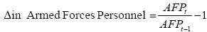
To examine if we get any kind of signaling consistency, we use the lagged change in Armed Forces Personnel to compare the impact of Military Expenditure (percentage of GDP), Arms Exports, Arms Imports, Military Expenditure (percentage of Central Government Expenditure), and GDP on the lagged change in Armed Forces Personnel, and define the lagged change in Armed Forces Personnel as:
 (1)
(1)
where the change in Armed Forces Personnel from year AFP t-1 to AFP t are computed. Δ in Armed Forces Personnel is the calculated change in percentage from year-to-year, where the first year of the Armed Forces Personnel at t is AFPt, and the next year Armed Forces Personnel t-1 is AFPt-1.
We construct a correlation analysis between Military Expenditure (percentage of GDP), Arms Exports, Arms Imports, Military Expenditure (percentage of Central Government Expenditure), GDP and the lagged change in Armed Forces Personnel (Hypothesis 1). Since Armed Forces Personnel is a calculated percentage of the total labor force for each country, we interpret it as scaled data, as we can easily quantify the change over time from country to country.
Since we are interested in whether an increase in the lagged change in Armed Forces Personnel is inversely related to GDP (meaning a positive change or increase in the lagged change in Armed Forces Personnel relative to GDP, the lower GDP and vice versa) and its impact on the other variables, we examine the Pearson’s correlation coefficient. Our interest lies in determining the effect on the sample (or confirmation of the inverse relationship between the lagged change in Armed Forces Personnel and GDP) as determined by the direction and significance level of the Pearson’s correlation coefficient.
We then run a regression analysis on the country specific data for the 22 countries in-sample by regressing the variables of Military Expenditure (percentage of GDP), Arms Exports (SIPRI trendindicator value), Arms Imports (SIPRI trend-indicator value), Military Expenditure (percentage of Central Government Expenditure) and GDP (constant in 2010 US Dollars) against the lagged change in Armed Forces Personnel. Thus, we define the regression as:
 (2)
(2)
where Δ AFPt is our dependent variable defined as the lagged change in Armed Forces Personnel at time t. βs are the regression coefficients, while X1 is Military Expenditure (percentage of GDP), X1 is Arms Exports (SIPRI trend-indicator value), X3 is Arms Import2 (SIPRI trend-indicator value), X4 is Military Expenditure (percentage of Central Government Expenditre), and X5 is GDP (constant in 2010 US Dollars). αi is the constant (intercept), while εi is the error term.
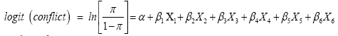
We use the statistically significant levels of the variables or consistent patterns within the data to construct a complex logistic regression to determine the likelihood of conflict within the in-sample countries. We define the logit model as
 (3)
(3)
therefore,
 (4)
(4)
 (5)
(5)
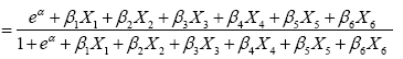
where π is the probability of conflict, α is the Y intercept, βs are the regression coefficients, and X1 is Military Expenditure (percentage of GDP), X2 is Arms Exports (SIPRI trend-indicator value), X3 is Arms Imports (SIPRI trend-indicator value), X4 is Military Expenditure (percentage of Central Government Expenditure), X5 is GDP (constant in 2010 US Dollars), and X6 is the lagged change in Armed Forces Personnel. We use the maximum likelihood method to estimate the α and βs following previous literature [20].
Upon completion of the correlation analysis, we regress the variables against the lagged change in Armed Forces Personnel for each in-sample country. Pending the statistical significance of those relationships and observed patterns country-wide (in-sample), we perform a logistic regression to determine the probability of conflict. We divide the data to examine the accuracy of the probabilities in determining conflict into two sub-samples. The first sub-sample (approximately 12 years) is analyzed to generate a baseline model of the probabilities, while the remaining data (approximately 13 years) is used to examine the consistency of the sample. We then test the probabilistic outcomes during the second sub-sample data on both the in-sample and out-of-sample data to determine accuracy (Hypothesis 2).
In our analyses (correlation, regression, and logistic regression), we follow the previous studies of Brock, Lakonishok, LeBaron, Andersen and Bollerslev to bootstrap confidence intervals for the coefficients and regressions, while using bias corrected accelerated (BCa) to select confidence intervals [21-23].
Correlation results
We run a correlation analysis on the world development indicators by taking Military Expenditure (percentage of GDP), Arms Exports (SIPRI trend-indicator value), Arms Imports (SIPRI trend-indicator value), Military Expenditure (percentage of Central Government Expenditure), and GDP (constant in 2010 US Dollars) with the lagged change in Armed Forces Personnel and selectively observe the Pearson’s correlation coefficient. Table 2 provides an example of the correlation analysis of Norway, as it generally meets the average profile of correlations reflected in the in-sample countries (including: Argentina, Australia, Belgium, Brazil, Canada, Chile, Denmark, Spain, United Kingdom, Ireland, Iran, Italy, Japan, South Korea, Malaysia, Netherlands, New Zealand, Portugal, Thailand, United States, and South Africa) (Table 2).
| Variables | 1 | 2 | 3 | 4 | 5 |
|---|---|---|---|---|---|
| Military Expenditure (% of GDP) | -- | -- | -- | -- | -- |
| Arms Exports (SIPRI Trend-Indicator Values) | -.285* | -- | -- | -- | -- |
| Arms Imports (SIPRI Trend-Indicator Values) | -.310 | -.067 | -- | -- | -- |
| Military Expenditure (% of Central Government Expenditures) | .930** | -.310* | -.279 | -- | -- |
| GDP (Constant in 2010 in US Dollars) | -.935** | .311* | .323 | -.984** | -- |
| Lagged change in Armed Forces Personnel (% of Total Labour Force) | .197 | -.288 | .055 | .140 | -.353 |
| ** Correlation is significant at the 0.01 level (2-tailed). * Correlation is significant at the 0.05 level (2-tailed) | |||||
Note: Out of the 22 countries analysed, Norway was selected for viewing as it generally met the average profile of the countries (including: Argentina, Australia, Belgium, Brazil, Canada, Chile, Denmark, Spain, United Kingdom, Ireland, Iran, Italy, Japan, South Korea, Malaysia, Netherlands, New Zealand, Portugal, Thailand, United States, and South Africa). Military Expenditure (percentage of Gross Domestic Product) is the military expenditure given in terms of the percentage of national Gross Domestic Product. Arms Exports is the SIPRI trend-indicator value, as is the Arms Imports (reported directly). Military Expenditure (percentage of Central Government Expenditure) is the percentage of military expenditure of each country’s central government expenditure. GDP is the reported Gross Domestic Product of each country reported in constant 2010 US Dollars. The lagged change in Armed Forces Personnel (1990-2015) is the calculated change from year 1 to year 2 and then subtracting 1 from the difference and defined as the percentage of armed forces personnel of each country’s total labour force.
Table 2: Correlation analysis for the variables of interest-This table reports the Pearson’s correlation coefficient and represents the intercorrelations of the variables used in this study.
Pearson’s correlation coefficients are summarized in Table 2 reflecting the intercorrelations of the variables (Norway). Consistent with expectations of the first hypothesis, all 22 countries exhibit a negative correlation between the lagged change in Armed Forces Personnel and GDP (confirming previous studies), although only 5 countries are statistically significant (Australia, Spain, Ireland, Japan, and the United States) at the p<0.05 level. We do find consistency in Military Expenditure (percentage of GDP) and Military Expenditure (percentage of Central Government Expenditure) as all but 1 of the countries exhibit positive correlations between the two variables at p<0.01 levels. The one exception is Japan (negative correlation) which also exhibits significance at the p<0.01 level. GDP (constant in 2010 US Dollars) and Military Expenditure (percentage of GDP) are negatively correlated in 21 of the 22 countries and significant at the p<0.01 level; the one exception is Japan, also significant at the p<0.01 level. GDP (constant in 2010 US Dollars) and Military Expenditure (percentage of Central Government Expenditure) are all negatively correlated for the 22 countries with 21 of the countries exhibiting significant at the p<0.01 level (exception: Spain). 17 of the 22 countries exhibit a negative relationship between Arms Exports (SIPRI trend-indicator value) and Military Expenditure (percentage of GDP) while 9 of the countries exhibit significant relationships at the p<0.05 or better. 11 of the countries exhibit negative relationships between Military Expenditure (percentage of GDP) and Arms Imports (SIPRI trend-indicator value) while only 5 relationships are significant at the p<0.05 or better.
Given the unique nature of the data, it is not surprising to find such inconsistency within the intervariable correlations. These inconsistencies imply that there might be more effects within those specific countries explaining variability within the data when isolated.
Regression results
Due to data constraints of Armed Forces Personnel (only available from 1990 to 2015), we analyze the world development indicators for the 22 countries selected by regressing Arms Exports (SIPRI trendindicator value), Arms Imports (SIPRI trend-indicator value) and GDP (constant in 2010 US Dollars) against the lagged change in Armed Forces Personnel (from 1990 to 2015). We eliminate Military Expenditure (percentage of GDP) as well as Military Expenditure (percentage of Central Government Expenditure) due to the correlation of Military Expenditure (percentage of GDP), Military Expenditure (percentage of Central Government Expenditure) and GDP (constant in 2010 US Dollars). Concerned with collinearity, we eliminate both Military Expenditure variables and use GDP (constant in 2010 US Dollars). Thus, our regression changes from equation (2) to reflect the following:
 (6)
(6)
where Δ AFPt (dependent variable) is defined as the lagged change in Armed Forces Personnel at time t. β1,t is the regression coefficient for Arms Exportt which is Arms Export (SIPRI trend-indicator value) at time t.β2,t is the regression coefficient for Arms Exportt which is Arms Imports (SIPRI trend-indicator value) at time t.β3,t is the regression coefficient for GDpt signifying GDP (constant in 2010 US Dollars) at time t. αi is the constant (intercept), while εi is the error term (Table 3).
| Period 1990-2015 |
Argentina | Australia | Belgium | Brazil | Canada |
|---|---|---|---|---|---|
| Constant (Intercept) | .398 | .287 | -.780 | 2.457 | .169 |
| Arms Exports (a) | -7.35E-9 | -2.46E-9* | -2.87E-10 | .000 | 7.62E-10* |
| Arms Imports (b) | 6.06E-9 | -5.88E-10 | -5.20E-9 | 2.10E-8 | -5.72E-11 |
| GDP (2010 USD) (c) | -9.75E-13 | -2.06E-13 | 1.74E-12 | -1.82E-12 | -2.21E-13* |
| Model | Y= -7.35E-9a + 6.06E-9b + -9.75E-13c + 0.398 |
Y= -2.46E-9a + -5.88E-10b + -2.06E-13c + 0.287 |
Y= -2.87E-10a + -5.20E-9b + 1.74E-12c +-0.780 |
Y.000a + 2.10E-8b + -1.82E-12c + 2.457 |
Y= 7.62E-10a + -5.72E-11b + -2.21E-13c + 0.169 |
| Predicted Y | 0.398 | 0.287 | -0.780 | 2.457 | 0.169 |
a: Regression analysis for the lagged change in armed forces personnel.
| Period 1990-2015 |
Chile | Denmark | Spain | United Kingdom | Ireland |
|---|---|---|---|---|---|
| Constant (Intercept) | -0.071 | 2.364 | 0.858* | 0.805 | 0.841 |
| Arms Exports (a) | -1.81E-10 | -1.39E-10 | 3.48E-11 | 6.41E-10 | -2.20E-9 |
| Arms Imports (b) | 5.22E-12 | 5.07EE-9 | -5.51E-9 | 2.63E-9 | -6.19E-11 |
| GDP (2010 USD) (c) | 3.45E-13 | -8.11E-12* | -6.29E-13 | -7.27E-13 | -3.36E-12 |
| Model | Y= -1.81E-10a + 5.22E-12b + 3.45E-13c + -0.071 |
Y=-.1.39E-10a + 5.07E-9b + -8.11E-12c + 2.364 |
Y= 3.48E-11a + -5.51E-9b + -6.29E-13c + 0.858 |
Y= 6.41E-10a + 2.63E-9b + -7.27E-13c + 0.805 |
Y= -2.20E-9a + -6.19E-11b + -3.36E-12c + 0.841 |
| Predicted Y | -0.071 | 2.364 | 0.858 | 0.805 | 0.841 |
b: Regression analysis for the lagged change in armed forces personnel.
| Period 1990-2015 |
Iran | Italy | Japan | South Korea | Malaysia |
|---|---|---|---|---|---|
| Constant (Intercept) | 3.501 | -1.392 | 3.762 | 0.270 | -0.110 |
| Arms Exports (a) | 1.55E-8* | 3.79E-11 | 1.38E-8 | -9.39E-10 | .000 |
| Arms Imports (b) | 6.14E-10 | -3.21E-8 | 3.49E-8 | -5.87E-11 | -2.59E-11 |
| GDP (2010 USD) (c) | -9.39E-12 | 7.37E-13 | -1.23E-12 | -1.84E-13 | 6.38E-13 |
| Model | Y= 1.55E-8a + 6.14E-10b + -9.39E-12c + 3.50 |
Y= 3.79E-11a + -3.21E-8b + 7.37E-13c + -1.392 |
Y= 1.38E-8a + 3.49E-8b + -1.23E-12c + 3.762 |
Y= -9.39E-10a + -5.87E-11b + -1.84E-13c + 0.270 |
Y= 0.000a + -2.59E-11b + 6.38E-13c + -0.110 |
| Predicted Y | 3.501 | -1.392 | 3.762 | 0.270 | -0.110 |
c: Regression analysis for the lagged change in armed forces personnel.
| Period 1990-2015 |
Netherlands | Norway | New Zealand | Portugal | Thailand |
|---|---|---|---|---|---|
| Constant (Intercept) | 0.041 | 0.695 | 1.99 | -0.997 | 3.72 |
| Arms Exports (a) | -1.03E-10 | -5.71E-10 | 3.39E-9 | .000 | .000 |
| Arms Imports (b) | -5.33E-11 | 3.45E-9 | -8.28E-11 | .000 | .000 |
| GDP (2010 USD) (c) | -2.69E-14 | -1.48E-12 | -1.07E-11 | 4.16E-12 | -1.16E-11 |
| Model | Y= -1.03E-10a + -5.33E-11b + -2.69E-14c +0.041 |
Y= -.5.71E-10a + 3.45E-9b + -1.48-12c + 0.695 |
Y= 3.39E-9a + -8.28E-11b + -1.07E-11c + 1.99 |
Y= 0.000a + 0.000b + 4.16E-12c + -0.997 |
Y= 0.000a + .000b + -1.16E-11c + 3.72 |
| Predicted Y | 0.041 | .695 | 1.99 | -.0997 | 3.72 |
d: Regression analysis for the lagged change in armed forces personnel.
| Period 1990-2015 |
United States | South Africa |
|---|---|---|
| Constant (Intercept) | 6.925 | 0.714 |
| Arms Exports (a) | 4.64E-10 | 2.71E-9 |
| Arms Imports (b) | 3.41E-9 | -5.57E-9 |
| GDP (2010 USD) (c) | -7.32E-13 | -2.76E-12 |
| Model | Y= 4.64E-10a + 3.41E-9b + -7.32E-13c + 6.92 |
Y= 2.71E-9a + -5.57E-9b + -2.76E-12c + 0.714 |
| Predicted Y | 6.925 | 0.714 |
e: Regression analysis for the lagged change in armed forces personnel.
Note: This table reports the regression analysis for the lagged change in Armed Forces Personnel from 1990 to 2015 for the 22 selected countries: Argentina, Australia, Belgium, Brazil, Canada, Chile, Denmark, Spain, United Kingdom, Ireland, Iran, Italy, Japan, South Korea, Malaysia, Netherlands, New Zealand, Norway, Portugal, Thailand, United States, and South Africa. The reported values for the Constant (Intercept), Predictor variables (gradient) of Arms Exports (SIPRI Trend-Indicator Value), Arms Imports (SIPRI Trend-Indicator Value), and GDP (constant 2010 in US Dollars), Model (Regression Line), and Predicted Y are shown. The independent variables (Arms Exports, Arms Imports, and GDP) have been previously defined. The lagged change in Armed Forces Personnel (dependent variable) is defined as the difference between the change in armed forces personnel (percentage of total labour force) from year 1 to year 2 and then subtracting 1 from the difference. Significance levels are reported as: *, **, *** 0.05, 0.01 and 0.001 levels, respectively.
Table 3: Regression analysis for the lagged change in armed forces personnel.
A summary of Table 3 includes the values for the Constant (Intercept), Predictor (gradient) values for Arms Exports (SIPRI trend-indicator value), Arms Imports (SIPRI trend-indicator value), and GDP (constant in 2010 US Dollars), Model (regression line), and the Predicted value of Y for the regression between Arms Exports, Arms Imports, and GDP against the lagged change in Arms Forces Personnel. We run regressions for the selected in-sample countries of: Argentina, Australia, Belgium, Brazil, Canada, Chile, Denmark, Spain, United Kingdom, Ireland, Iran, Italy, Japan, South Korea, Malaysia, Netherlands, New Zealand, Norway, Portugal, Thailand, United States, and South Africa.
We find regressions between Arms Exports, Arms Imports, GDP and the lagged change in Armed Forces Personnel are mostly positive, with the exceptions being Belgium, Chile, Italy, and Portugal. Unsurprisingly, very few interactions are statistically significant. Given the inherent complications of comparing country specific data, we are not expecting many statistically significant interactions, but focus on emerging patterns within the data.
However, there are a couple of statistically significant relationships: Australia (Arms Exports significantly negative at the p<0.05 level), Canada (Arms Exports significantly positive at the p<0.05 level), Spain (Constant significantly positive at the p<0.05 level), and Iran (Arms Exports significantly positive at the p<0.05 level). The Arms Exports interaction is split between 9 countries reflecting positive values, 9 countries reflecting negative values, and 4 countries reflecting values of 0.000. Arms Imports interaction is split between 11 countries reflecting negative values, 9 countries reflecting positive values, and 2 countries reflecting values of 0.000. The GDP is more consistent, as 17 countries reflect negative interactions, while 5 countries reflect a positive interaction (Belgium, Chile, Italy, Malaysia, and Portugal).2
Logit results
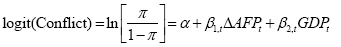
Given our findings in the correlation analysis and the regression analysis, we reduce the world development indicators in the logistic regression to include the lagged change in Armed Forces Personnel and GDP with the outcome variable of Conflict (coded as 1=Yes and 0=No).3 We define the adjusted logit model as:
 (7)
(7)
therefore,
 (8)
(8)
 (9)
(9)
where π is the probability of Conflict, α is the Y intercept, β1,t is the regression coefficient for Δ AFPt defined as the lagged percentage change in Armed Forces Personnel at time t, while β2,t is the regression coefficient for GDpt defined as the Gross Domestic Product (constant in 2010 US Dollars) at time t. Consistent with equations (4) and (5), α and βs are estimated by the maximum likelihood method [20].
Based on the Omnibus Tests of Model Coefficients, we eliminate the variable β2,t GDpt (defined as the Gross Domestic Product, constant in 2010 US Dollars), thus leaving the lagged change in Armed Forces Personnel (Δ AFPt) as the only independent variable of the likelihood of conflict.4 We eliminate all but Australia, Canada, Chile, Ireland, Italy, South Korea, Malaysia, Norway, New Zealand, Portugal, Thailand, and South Africa for the in-sample countries due to minor discrepancies within the dataset affecting baseline model development (Table 4).
| Predictor | β | SE β | Wald’s χ2 | df | p | е^β(odds ratio) |
|---|---|---|---|---|---|---|
| Constant | -2.371 | 1.051 | 5.090 | 1 | 0.013 | 0.093 |
| Δ in Armed Forces Personnel | 3.198 | 9.680 | 0.109 | 1 | 0.406 | 24.488 |
| Test | -- | -- | χ2 | df | p | -- |
| Overall Model Evaluation | -- | -- | -- | -- | -- | -- |
| Likelihood Ratio Test | -- | -- | 0.103 | 1 | 0.748 | -- |
| Goodness-of-fit Test | -- | -- | -- | -- | -- | -- |
| Hosmer & Lemeshow | -- | -- | 2.167 | 8 | 0.975 | -- |
|
Cox and Snell R2=0.009 |
||||||
4a: Country-Australia
| Predictor | β | SE β | Wald’s χ2 | df | p | е^β(odds ratio) |
|---|---|---|---|---|---|---|
| Constant | -2.451 | 1.093 | 5.034 | 1 | 0.016 | 0.086 |
| Δ in Armed Forces Personnel | 3.206 | 6.444 | .248 | 1 | 0.104 | 24.692 |
| Test | -- | -- | χ2 | df | p | -- |
| Overall Model Evaluation | -- | -- | -- | -- | -- | -- |
| Likelihood Ratio Test | -- | -- | 0.216 | 1 | 0.642 | -- |
| Goodness-of-fit Test | -- | -- | -- | -- | -- | -- |
| Hosmer & Lemeshow | -- | -- | 1.715 | 8 | 0.989 | -- |
|
Cox and Snell R2=0.018 |
||||||
4b: Country-Canada.
| Predictor | β | SE β | Wald’s χ2 | df | p | е^β(odds ratio) |
|---|---|---|---|---|---|---|
| Constant | -4.398 | 2.689 | 2.675 | 1 | 0.003 | 0.012 |
| Δ in Armed Forces Personnel | -33.267 | 27.821 | 1.430 | 1 | 0.007 | 0.001 |
| Test | χ2 | df | p | -- | ||
| Overall Model Evaluation | -- | -- | -- | -- | -- | -- |
| Likelihood Ratio Test | -- | -- | 2.113 | 1 | 0.146 | -- |
| Goodness-of-fit Test | -- | -- | -- | -- | -- | -- |
| Hosmer & Lemeshow | -- | -- | 0.267 | 8 | 0.999 | -- |
|
Cox and Snell R2=0.161 |
||||||
4c: Country-Chile
| Predictor | β | SE β | Wald’s χ2 | df | p | е^β(odds ratio) |
|---|---|---|---|---|---|---|
| Constant | -2.431 | 1.073 | 5.127 | 1 | 0.019 | 0.088 |
| Δ in Armed forces personnel | 1.656 | 5.802 | .081 | 1 | 0.528 | 5.239 |
| Test | -- | -- | χ2 | df | p | -- |
| Overall model evaluation | -- | -- | -- | -- | -- | -- |
| Likelihood ratio test | -- | -- | 0.077 | 1 | 0.781 | -- |
| Goodness-of-fit Test | -- | -- | -- | -- | -- | |
| Hosmer & Lemeshow | -- | -- | 11.554 | 8 | 0.173 | -- |
|
Cox and Snell R2=0.006 |
||||||
4d: Country-Ireland
| Predictor | β | SE β | Wald’s χ2 | df | p | е^β(odds ratio) |
|---|---|---|---|---|---|---|
| Constant | -2.441 | 1.095 | 4.969 | 1 | 0.022 | 0.087 |
| Δ in Armed Forces Personnel | -3.241 | 18.125 | 0.032 | 1 | 0.359 | 0.039 |
| Test | -- | -- | χ2 | df | p | -- |
| Overall Model Evaluation | -- | -- | -- | -- | -- | -- |
| Likelihood Ratio Test | -- | -- | 0.033 | 1 | 0.855 | -- |
| Goodness-of-fit Test | -- | -- | -- | -- | -- | -- |
| Hosmer & Lemeshow | -- | -- | 2.707 | 8 | 0.951 | -- |
|
Cox and Snell R2=0.003 |
||||||
4e: Country-Italy
| Predictor | β | SE β | Wald’s χ2 | df | p | е^β(odds ratio) |
|---|---|---|---|---|---|---|
| Constant | 1.339 | 1.146 | 1.365 | 1 | 0.051 | 3.814 |
| Δ in Armed forces personnel | -13.809 | 16.324 | 0.716 | 1 | 0.069 | 0.001 |
| Test | -- | -- | χ2 | df | p | -- |
| Overall model evaluation | -- | -- | -- | -- | -- | -- |
| Likelihood ratio test | -- | -- | 4.012 | 1 | 0.045 | -- |
| Goodness-of-fit Test | -- | -- | -- | -- | -- | -- |
| Hosmer & Lemeshow | -- | -- | 6.163 | 7 | 0.521 | -- |
|
Cox and Snell R2=0.360 |
||||||
4f: Country-South Korea
| Predictor | β | SE β | Wald’s χ2 | df | p | е^β(odds ratio) |
|---|---|---|---|---|---|---|
| Constant | -2.061 | 1.414 | 2.124 | 1 | 0.061 | 0.127 |
| Δ in Armed forces personnel | 8.714 | 28.079 | .096 | 1 | 0.460 | 6085.538 |
| Test | -- | χ2 | df | p | -- | |
| Overall model evaluation | -- | -- | -- | -- | -- | -- |
| Likelihood ratio test | -- | -- | 0.096 | 1 | 0.757 | -- |
| Goodness-of-fit Test | -- | -- | -- | -- | -- | -- |
| Hosmer & Lemeshow | -- | -- | 11.442 | 8 | 0.178 | -- |
|
Cox and Snell R2=0.008 |
||||||
4g: Country-Malaysia
| Predictor | β | SE β | Wald’s χ2 | df | p | е^β(odds ratio) |
|---|---|---|---|---|---|---|
| Constant | -2.441 | 1.095 | 4.969 | 1 | 0.022 | 0.077 |
| Δ in Armed forces personnel | -3.241 | 18.125 | 0.032 | 1 | 0.359 | 0.001 |
| Test | -- | -- | χ2 | df | p | -- |
| Overall model evaluation | -- | -- | -- | -- | -- | -- |
| Likelihood ratio test | -- | -- | 0.731 | 1 | .393 | -- |
| Goodness-of-fit Test | -- | -- | -- | -- | -- | -- |
| Hosmer & Lemeshow | -- | -- | 8.437 | 8 | 0.392 | -- |
|
Cox and Snell R2=0.059 |
||||||
4h: Country-Norway
| Predictor | β | SE β | Wald’s χ2 | df | p | е^β(odds ratio) |
|---|---|---|---|---|---|---|
| Constant | -1.999 | 1.844 | 1.174 | 1 | 0.088 | 0.136 |
| Δ in Armed forces personnel | 14.728 | 60.642 | 0.059 | 1 | 0.463 | 2489292.6 |
| Test | -- | χ2 | df | p | -- | |
| Overall model evaluation | -- | -- | -- | -- | -- | -- |
| Likelihood ratio test | -- | -- | 0.065 | 1 | 0.798 | -- |
| Goodness-of-fit Test | -- | -- | -- | -- | -- | -- |
| Hosmer & Lemeshow | -- | -- | 11.619 | 8 | 0.169 | -- |
|
Cox and Snell R2=0.005 |
||||||
4i: Country-New Zealand
| Predictor | β | SE β | Wald’s χ2 | df | p | е^β(odds ratio) |
|---|---|---|---|---|---|---|
| Constant | -2.453 | 1.261 | 3.748 | 1 | 0.024 | 0.086 |
| Δ in Armed forces personnel | -6.809 | 24.416 | 0.078 | 1 | 0.251 | 0.001 |
| Test | -- | -- | χ2 | df | p | -- |
| Overall model evaluation | -- | -- | -- | -- | -- | -- |
| Likelihood ratio test | -- | -- | 0.270 | 1 | 0.603 | -- |
| Goodness-of-fit Test | -- | -- | -- | -- | -- | -- |
| Hosmer & Lemeshow | -- | -- | 10.538 | 8 | 0.229 | -- |
|
Cox and Snell R2=0.022 |
||||||
4j: Country-Portugal
| Predictor | β | SE β | Wald’s χ2 | df | p | е^β(odds ratio) |
|---|---|---|---|---|---|---|
| Constant | -2.135 | 1.060 | 4.058 | 1 | 0.044 | 0.118 |
| Δ in Armed forces personnel | -0.426 | 1.588 | 0.072 | 1 | 0.373 | 0.653 |
| Test | -- | χ2 | df | p | -- | |
| Overall model evaluation | -- | -- | -- | -- | -- | -- |
| Likelihood ratio test | -- | -- | 0.140 | 1 | 0.708 | -- |
| Goodness-of-fit Test | -- | -- | -- | -- | -- | -- |
| Hosmer & Lemeshow | -- | -- | 9.350 | 8 | 0.314 | -- |
|
Cox and Snell R2=0.014 |
||||||
4k: Country-Thailand.
| Predictor | β | SE β | Wald’s χ2 | df | p | е^β(odds ratio) |
|---|---|---|---|---|---|---|
| Constant | -2.499 | 1.344 | 3.454 | 1 | 0.013 | 0.082 |
| Δ in Armed forces personnel | -7.155 | 34.336 | 0.043 | 1 | 0.003 | 0.001 |
| Test | -- | -- | χ2 | df | p | -- |
| Overall model evaluation | -- | -- | -- | -- | -- | -- |
| Likelihood ratio test | -- | -- | 0.144 | 1 | 0.704 | -- |
| Goodness-of-fit Test | -- | -- | -- | -- | -- | -- |
| Hosmer & Lemeshow | -- | -- | 11.198 | 8 | 0.191 | -- |
|
Cox and Snell R2=0.012 |
||||||
4l: Country-South Africa
Note: This table reports the logistic regression analysis for the in-sample countries of Australia, Canada, Chile, Ireland, Italy, South Korea, Malaysia, Norway, New Zealand, Portugal, Thailand, and South Africa for the years of 1990-2001. We include the Predictors (Constant and the lagged change in Armed Forces Personnel) and report the coefficients, chi-squares, degrees of freedom, significance, and the odds ratio. The lagged change in Armed Forces Personnel (Δ in Armed Forces Personnel) is calculated as the change from year 1 to year 2 and then subtracting 1 from the difference and defined as the percentage of armed forces personnel of each country’s total labour force. We also report the overall model evaluation and goodness-of-fit test for each country (as well as the Cox and Snell R2 and Nagelkerke R2 as supplementary measures). Logistic Regression Analysis (1990-2001).
Table 4: Logistic regression analysis for in-sample countries.
Table 4 summarizes the logistic regression analysis for the insample countries of Australia, Canada, Chile, Ireland, Italy, South Korea, Malaysia, Norway, New Zealand, Portugal, Thailand, and South Africa for the years of 1990-2001. We include the Predictors (Constant and the lagged change in Armed Forces Personnel) and report the coefficients, chi-squares, degrees of freedom, significance, and the odds ratio. We also report the overall model evaluation and goodness-of-fit test for each country (as well as the Cox and Snell R2 and Nagelkerke R2 as supplementary measures).
We run logistic regressions on each of the countries independently and find mixed results. Given the data challenges previously analyzed, expectations generally match those of the previous models. We find that the models’ overall evaluation (likelihood ratio tests) do not perform very well (consistently).5 However, we do find that the goodness-of-fit test yield insignificant results (p >0.05) suggesting that each model fit the data reasonably well (or at least the null hypothesis of a good model fit was obtainable) [21]. The predictor variable of the lagged change in Armed Forces Personnel is significant for the countries of Chile (p<0.05) and South Africa (p<0.05), while most of the Constants are significant (p<0.05) for the in-sample countries with the exceptions of South Korea, Malaysia, and New Zealand (Table 5).
| Year | Δ in Armed Forces Personnel β=3.198 |
Intercept = -2.371 |
Predicted Probability of Conflict | Actual Outcome 1=Yes, 0=No |
|---|---|---|---|---|
| 1990 | 0.0093 | -2.371 | 0.1924 | 0 |
| 1991 | -0.0214 | -2.371 | 0.1744 | 0 |
| 1992 | 0.0130 | -2.371 | 0.1947 | 0 |
| 1993 | -0.0250 | -2.371 | 0.1724 | 0 |
| 1994 | 0.2289 | -2.371 | 0.3884 | 0 |
| 1995 | 0.0073 | -2.371 | 0.1912 | 0 |
| 1996 | -0.1824 | -2.371 | 0.1042 | 0 |
| 1997 | -0.0091 | -2.371 | 0.1814 | 0 |
| 1998 | -0.1165 | -2.371 | 0.1287 | 0 |
| 1999 | -0.0029 | -2.371 | 0.1815 | 0 |
| 2000 | -0.1430 | -2.371 | 0.1182 | 0 |
| 2001 | -0.0216 | -2.371 | 0.1743 | 0 |
a: Country-Australia.
| Year | Δ in Armed Forces Personnel β=3.206 |
Intercept = -2.451 |
Predicted Probability of Conflict | Actual Outcome 1=Yes, 0=No |
|---|---|---|---|---|
| 1990 | 0.0545 | -2.451 | 0.2054 | 0 |
| 1991 | -0.0859 | -2.451 | 0.1309 | 0 |
| 1992 | -0.0570 | -2.451 | 0.1436 | 0 |
| 1993 | 0.0193 | -2.451 | 0.1834 | 0 |
| 1994 | 0.3663 | -2.451 | 0.5579 | 0 |
| 1995 | -0.0530 | -2.451 | 0.1455 | 0 |
| 1996 | -0.0287 | -2.451 | 0.1572 | 0 |
| 1997 | -0.0060 | -2.451 | 0.1691 | 0 |
| 1998 | -0.0365 | -2.451 | 0.1534 | 0 |
| 1999 | -0.0360 | -2.451 | 0.1536 | 0 |
| 2000 | -0.1760 | -2.451 | 0.0981 | 0 |
| 2001 | -0.0500 | -2.451 | 0.1469 | 0 |
b: Country-Canada.
| Year | Δ in Armed Forces Personnel β=-33.267 |
Intercept = -4.398 |
Predicted Probability of Conflict | Actual Outcome 1=Yes, 0=No |
|---|---|---|---|---|
| 1990 | -0.0973 | -4.398 | 0.6266 | 0 |
| 1991 | -0.0275 | -4.398 | 0.0613 | 0 |
| 1992 | -0.0567 | -4.398 | 0.1621 | 0 |
| 1993 | -0.0477 | -4.398 | 0.1202 | 0 |
| 1994 | 0.3914 | -4.398 | 0.0001 | 0 |
| 1995 | -0.0163 | -4.398 | 0.0424 | 0 |
| 1996 | -0.1311 | -4.398 | 1.9298 | 0 |
| 1997 | 0.0384 | -4.398 | 0.0069 | 0 |
| 1998 | -0.0111 | -4.398 | 0.0356 | 0 |
| 1999 | 0.0102 | -4.398 | 0.0175 | 0 |
| 2000 | -0.0332 | -4.398 | 0.0743 | 0 |
| 2001 | -0.0194 | -4.398 | 0.0468 | 0 |
c: Country-Chile.
| Year | Δ in Armed Forces Personnel β=1.656 |
Intercept = -2.431 |
Predicted Probability of Conflict | Actual Outcome 1=Yes, 0=No |
|---|---|---|---|---|
| 1990 | 0.0454 | -2.431 | 0.1896 | 0 |
| 1991 | 0.1192 | -2.431 | 0.2143 | 0 |
| 1992 | -0.0131 | -2.431 | 0.1721 | 0 |
| 1993 | -0.0144 | -2.431 | 0.1718 | 0 |
| 1994 | 0.4204 | -2.431 | 0.3529 | 0 |
| 1995 | 0.1024 | -2.431 | 0.2084 | 0 |
| 1996 | -0.0388 | -2.431 | 0.1650 | 0 |
| 1997 | -0.0991 | -2.431 | 0.1493 | 0 |
| 1998 | -0.0877 | -2.431 | 0.1521 | 0 |
| 1999 | -0.0881 | -2.431 | 0.1520 | 0 |
| 2000 | -0.3034 | -2.431 | 0.1064 | 0 |
| 2001 | -0.0399 | -2.431 | 0.1646 | 0 |
d: Country-Ireland.
| Year | Δ in Armed Forces Personnel β=-3.241 |
Intercept = -2.441 |
Predicted Probability of Conflict | Actual Outcome 1=Yes, 0=No |
|---|---|---|---|---|
| 1990 | -0.0188 | -2.441 | 0.1851 | 0 |
| 1991 | -0.0183 | -2.441 | 0.1848 | 0 |
| 1992 | -0.0168 | -2.441 | 0.1839 | 0 |
| 1993 | -0.0176 | -2.441 | 0.1843 | 0 |
| 1994 | 0.1596 | -2.441 | 0.1038 | 0 |
| 1995 | -0.0500 | -2.441 | 0.1770 | 0 |
| 1996 | -0.0115 | -2.441 | 0.1807 | 0 |
| 1997 | -0.0005 | -2.441 | 0.1744 | 0 |
| 1998 | -0.1377 | -2.441 | 0.2721 | 0 |
| 1999 | -0.0147 | -2.441 | 0.1826 | 0 |
| 2000 | -0.0091 | -2.441 | 0.1793 | 0 |
| 2001 | -0.0088 | -2.441 | 0.1792 | 0 |
e: Country-Italy.
| Year | Δ in Armed Forces Personnel β=-13.809 |
Intercept = 1.339 |
Predicted Probability of Conflict | Actual Outcome 1=Yes, 0=No |
|---|---|---|---|---|
| 1990 | 0.4406 | 1.339 | 0.0174 | 1 |
| 1991 | -1.00 | 1.339 | 758.093 | 1 |
| 1992 | -1.00 | 1.339 | 758.093 | 1 |
| 1993 | -1.00 | 1.339 | 758.093 | 1 |
| 1994 | -1.00 | 1.339 | 758.093 | 1 |
| 1995 | -0.0521 | 1.339 | 15.6695 | 1 |
| 1996 | -0.0742 | 1.339 | 21.2499 | 1 |
| 1997 | -0.0685 | 1.339 | 19.6474 | 1 |
| 1998 | -0.0685 | 1.339 | 18.9278 | 1 |
| 1999 | -0.0530 | 1.339 | 15.8665 | 1 |
| 2000 | -0.0206 | 1.339 | 10.1471 | 1 |
| 2001 | 0.0504 | 1.339 | 3.8026 | 1 |
f: Country-S. Korea.
| Year | Δ in Armed Forces Personnel β=8.714 |
Intercept = -2.061 |
Predicted Probability of Conflict | Actual Outcome 1=Yes, 0=No |
|---|---|---|---|---|
| 1990 | -0.0327 | -2.061 | 1.8935 | 1 |
| 1991 | -0.1058 | -2.061 | 6.7343 | 1 |
| 1992 | -0.6027 | -2.061 | 3.1575 | 0 |
| 1993 | -0.0688 | -2.061 | 3.5087 | 0 |
| 1994 | -0.0589 | -2.061 | 2.9564 | 0 |
| 1995 | -0.0477 | -2.061 | 2.4377 | 0 |
| 1996 | -0.0444 | -2.061 | 2.3066 | 0 |
| 1997 | 0.0214 | -2.061 | 0.8343 | 0 |
| 1998 | -0.0254 | -2.061 | 1.6798 | 0 |
| 1999 | -0.0864 | -2.061 | 4.7818 | 0 |
| 2000 | -0.0313 | -2.061 | 1.8505 | 0 |
| 2001 | 0.0202 | -2.061 | 0.8480 | 0 |
g: Country-Malaysia.
| Year | Δ in Armed Forces Personnel β=-19.743 |
Intercept = -2.562 |
Predicted Probability of Conflict | Actual Outcome 1=Yes, 0=No |
|---|---|---|---|---|
| 1990 | -0.0282 | -2.562 | 0.2681 | 0 |
| 1991 | -0.0308 | -2.562 | 0.2821 | 0 |
| 1992 | -0.0321 | -2.562 | 0.2895 | 0 |
| 1993 | -0.0320 | -2.562 | 0.2889 | 0 |
| 1994 | 0.7444 | -2.562 | 0.0001 | 0 |
| 1995 | 0.1003 | -2.562 | 0.0216 | 0 |
| 1996 | 0.1841 | -2.562 | 0.0042 | 0 |
| 1997 | 0.0240 | -2.562 | 0.0965 | 0 |
| 1998 | -0.0213 | -2.562 | 0.2340 | 0 |
| 1999 | -0.0180 | -2.562 | 0.2197 | 0 |
| 2000 | -0.0617 | -2.562 | 0.5164 | 0 |
| 2001 | 0.0399 | -2.562 | 0.0706 | 0 |
h: Country-Norway.
| Year | Δ in Armed Forces Personnel β=14.728 |
Intercept = -1.999 |
Predicted Probability of Conflict | Actual Outcome 1=Yes, 0=No |
|---|---|---|---|---|
| 1990 | -0.0247 | -1.999 | 0.1883 | 0 |
| 1991 | -0.0741 | -1.999 | 0.0909 | 0 |
| 1992 | -0.0369 | -1.999 | 0.1574 | 0 |
| 1993 | -0.0128 | -1.999 | 0.2243 | 0 |
| 1994 | -0.0088 | -1.999 | 0.2381 | 0 |
| 1995 | -0.0235 | -1.999 | 0.1917 | 0 |
| 1996 | -0.0230 | -1.999 | 0.1931 | 0 |
| 1997 | -0.0109 | -1.999 | 0.2307 | 0 |
| 1998 | -0.0256 | -1.999 | 0.1859 | 0 |
| 1999 | -.0603 | -1.999 | 0.1115 | 0 |
| 2000 | -0.0425 | -1.999 | 0.1449 | 0 |
| 2001 | -0.0094 | -1.999 | 0.2359 | 0 |
i: Country-New Zealand.
| Year | Δ in Armed Forces Personnel β=--6.809 |
Intercept = -2.453 |
Predicted Probability of Conflict | Actual Outcome 1=Yes, 0=No |
|---|---|---|---|---|
| 1990 | -0.0291 | -2.453 | 0.2098 | 0 |
| 1991 | -0.0274 | -2.453 | 0.2074 | 0 |
| 1992 | -0.0303 | -2.453 | 0.2114 | 0 |
| 1993 | -0.0312 | -2.453 | 0.2128 | 0 |
| 1994 | 0.7174 | -2.453 | 0.0013 | 0 |
| 1995 | 0.2013 | -2.453 | 0.0437 | 0 |
| 1996 | -0.0286 | -2.453 | 0.2091 | 0 |
| 1997 | -0.0287 | -2.453 | 0.2092 | 0 |
| 1998 | -0.0289 | -2.453 | 0.2095 | 0 |
| 1999 | -0.0291 | -2.453 | 0.2098 | 0 |
| 2000 | -0.0726 | -2.453 | 0.2821 | 0 |
| 2001 | -0.0289 | -2.453 | 0.2095 | 0 |
j: Country-Portugal.
| Year | Δ in Armed Forces Personnel β=-.0426 |
Intercept = -2.135 |
Predicted Probability of Conflict | Actual Outcome 1=Yes, 0=No |
|---|---|---|---|---|
| 1990 | -0.0167 | -2.135 | 0.2382 | 0 |
| 1991 | -0.0167 | -2.135 | 0.2382 | 0 |
| 1992 | -0.0167 | -2.135 | 0.2382 | 0 |
| 1993 | -0.0167 | -2.135 | 0.2382 | 0 |
| 1994 | 4.8956 | -2.135 | 0.0294 | 0 |
| 1995 | 0.2786 | -2.135 | 0.2100 | 0 |
| 1996 | -0.5748 | -2.135 | 0.3021 | 0 |
| 1997 | -0.0212 | -2.135 | 0.2386 | 0 |
| 1998 | -0.0237 | -2.135 | 0.2389 | 0 |
| 1999 | -0.3132 | -2.135 | 0.2702 | 0 |
| 2000 | -0.0307 | -2.135 | 0.2396 | 0 |
| 2001 | -0.0340 | -2.135 | 0.2399 | 0 |
k: Country-Thailand.
| Year | Δ in Armed Forces Personnel β=-7.155 |
Intercept = -2.499 |
Predicted Probability of Conflict | Actual Outcome 1=Yes, 0=No |
|---|---|---|---|---|
| 1990 | -0.0247 | -2.499 | 0.2177 | 0 |
| 1991 | -0.0249 | -2.499 | 0.2180 | 0 |
| 1992 | -0.0252 | -2.499 | 0.2186 | 0 |
| 1993 | -0.0262 | -2.499 | 0.2201 | 0 |
| 1994 | 0.3985 | -2.499 | 0.0101 | 0 |
| 1995 | -0.0271 | -2.499 | 0.2215 | 0 |
| 1996 | -0.0282 | -2.499 | 0.2233 | 0 |
| 1997 | -0.0289 | -2.499 | 0.2244 | 0 |
| 1998 | -0.0289 | -2.499 | 0.2244 | 0 |
| 1999 | -0.0286 | -2.499 | 0.2239 | 0 |
| 2000 | -0.0254 | -2.499 | 0.2188 | 0 |
| 2001 | -0.0254 | -2.499 | 0.2188 | 0 |
l: Country-South Africa.
Note: This table represents the predicted probability of Conflict for the selected countries (in-sample): Australia, Canada, Chile, Ireland, Italy, South Korea, Malaysia, Norway, New Zealand, Portugal, Thailand, and South Africa. The in-sample countries represent the years 1990-2001 (for the first sub-sample), and reflects the lagged change in Armed Forces Personnel (Δ in Armed Forces Personnel) calculated as the change from year 1 to year 2 and then subtracting 1 from the difference and defined as the percentage of armed forces personnel of each country’s total labour force, the Intercept (Constant), Predicted Probability of Conflict, and the Actual Outcome (1=Yes, 0=No), where ‘Yes’ indicates that the country experienced conflict. Predicted Probability of Conflict (1990-2001).
Table 5: Predicted probability of conflict.
Table 5 summarizes the values representing the predicted probability of Conflict for the selected countries (in-sample), for the years 1990-2001 and includes the lagged change in Armed Forces Personnel, the Constant (Intercept), Predicted Probability of Conflict, and the Actual Outcome (coded 1=Yes, 0=No), where ‘Yes’ equates to the country experiencing conflict.
We find the predicted probabilities of Conflict do a good job with the in-sample countries of predicting Conflict as well as predicting no Conflict for the years of 1990 to 2001. When using the cut-off score of 1.0 (meaning definitive Conflict imminent) predicted probability of conflict, the in-sample population was correct 93% of the time (134/144). There are 9 false positives (forecasted Conflict that did not transpire), and 1 false negative (miss of actual Conflict). 8 of the false positives are for the country of Malaysia, implying that the predicted probability of conflict is not a good indicator for this country. However, given the unique political situation exhibited in Malaysia during the sample years, it is not surprising that the lagged change in Armed Forces Personnel within the logistic regression would imply that conflict is on the horizon. The additional false positive is from Chile (1996). The false negative is the first year of the analysis in the sample (1990) for South Korea (Table 6).
| In-Sample 1990-2001 | |||
|---|---|---|---|
| Observed | Predicted Yes |
Predicted No | % Correct |
| Yes | 13 | 9 | 59.1% |
| No | 1 | 121 | 99.2% |
| Overall % Correct | -- | -- | 93.1% |
| Sensitivity=13/(13+9)=59.1%, Specificity=121/(1+121)=99.2%, False Positives=1/(1+13)=7.1%, False Negatives=9/(9+121)=6.9% | |||
| In-Sample 2002-2015 | |||
| Observed | Predicted Yes |
Predicted No | % Correct |
| Yes | 31 | 8 | 79.5% |
| No | 13 | 104 | 88.9% |
| Overall % Correct | -- | -- | 86.5% |
| Sensitivity=31/(31+8)=79.5%, Specificity=104/(13+104)=88.9%, False Positives=13/(13+31)=29.5%, False Negatives=8/(8+104)=7.1% | |||
| Out-of-Sample 2002-2015 | |||
| Observed | Predicted Yes |
Predicted No | % Correct |
| Yes | 118 | 79 | 59.9% |
| No | 28 | 1881 | 98.5% |
| Overall % Correct | 94.9% | ||
| Sensitivity=118/(118+79)=59.9%, Specificity=1881/(28+1881)=98.5%, False Positives=28/(28+118)=19.2%, False Negatives=79/(79+1881)=4.03% | |||
Note: The observed and predicted frequencies for Conflict by logistic regression with the Cut-off of 1.0 for the in-sample1 countries for the period of 1990-2001, as well as the in-sample countries for the period of 2002-2015 and the out-of-sample2 countries for the period 2002-2015.
Table 6: Observed and predicted frequencies for conflict.
Table 6 represents the observed and predicted frequencies for conflict for the in-sample countries of the first sub-sample (1990-2001), the in-sample countries of the second sub-sample (2002-2015), and the out-of-sample countries6 (2002-2015). In support of Hypothesis 2, all three samples exhibit correct percentages over 85% (predicted frequency for conflict). The in-sample countries show a slight decrease in accuracy when comparing the first sub-sample with the second subsample (93.1% vs. 86.5%). False positives drastically rose from the first sub-sample to the second sub-sample (7.1% vs. 29.5%), while false negatives remained somewhat similar (6.9% vs. 7.1%). The out-ofsample countries exhibit surprisingly accurate predicted frequency for conflict (94.9% overall). False positives are a little less than the second sub-sample (in-sample countries) at 19.2%, while false negatives are slightly lower (4.01%).
This study reflects unique information World Development indicators possess in signaling conflict. Using World Development indicators from 1960 to 2015, we find that the lagged change in Armed Forces Personnel can with greater than 85% overall accuracy (in both in-sample and out-of-sample countries) signal conflict.
While we find support for both hypotheses, the lack of statistically significant relationships poses challenges. As the SIPRI data continues to progress, we expect further improvements of comparability from country-to-country and further support internationally to ensure better accuracy of the data within. As development continues, a more robust dataset will enhance future studies, plausibly to verify statistically significant relationships of this work. Due to data limitations, the statistical analyses are prone to inherent limitations [24].
It is also important to note that while extant literature does not offer specific guidance to the sample size of a logistic regression, the recommended sample size is 100 or more with a variable number as a function of predictors [25]. Surprisingly, the out-of-sample countries exhibit an overall accuracy of 94.9%, outperforming the in-sample countries (in both sub-samples) with a limited predictor.
We attribute the accuracy of the out-of-sample findings to the larger amount of countries not exhibiting conflict (artificially boosting accuracy). A better predictor of the accuracy is the sensitivity of the logistic regression, although all three analyses exhibited better than 50% accuracy. This reflects the signaling validity within the model, and the valuable content of the lagged change in Armed Forces Personnel. In isolation, the predictability of conflict based on the lagged change in Armed Forces Personnel is not a stable metric. However, combined with already established metrics, this is another tool to help in dismantling conflict before it arises.
Future studies would benefit from a more robust dataset for both in-sample and out-of-sample countries. As the dataset becomes more robust, accuracy in predicting or signaling conflict will also become more stable as more predictors can be added to the logistic regression. The findings of this study generally support previous literature but differentiate by focusing on the lagged change in Armed Forces Personnel as a predictor of conflict.
1 In-Sample Countries: Australia, Canada, Chile, Ireland, Italy, South Korea, Malaysia, Norway, New Zealand, Portugal, Thailand, and South Africa.
2 Out-of-Sample Countries: Aruba, Afghanistan, Angola, Andorra, United Arab Emirates, Argentina, Antigua and Barbuda, Australia, Austria, Azerbaijan, Burundi, Belgium, Benin, Burkina Faso, Bangladesh, Bulgaria, Bahrain, Bahamas, Bosnia and Herzegovina, Belize, Bermuda, Bolivia, Brazil, Barbados, Brunei Darussalam, Bhutan, Botswana, Central African Republic, Channel Islands, China, Ivory Coast, Cameroon, Congo, Comoros, Cabo Verde, Costa Rica, Cayman Islands, Cyprus, Czech Republic, Germany, Dominica, Denmark, Dominica Republic, Algeria, Ecuador, Egypt, Eritrea, Spain, Estonia, Ethiopia, Finland, Fiji, Micronesia, Gabon, United Kingdom, Georgia, Gibraltar, Guinea, Gambia, Greenland, Guam, Guyana, Honduras, Croatia, Haiti, Hungary, Indonesia, Isle of Man, Iran, Iraq, Israel, Jamaica, Jordan, Kazakhstan, Kenya, Kyrgyz Republic, St. Kitts and Nevis, Kuwait, Lao, Lebanon, Liberia, St. Lucia, Liechtenstein, Sri Lanka, Lesotho, Lithuania, Luxembourg, Morocco, Monaco, Madagascar, Maldives, Mexico, Marshall Islands, Macedonia, Mali, Malta, Myanmar, Mongolia, Northern Mariana Islands, Mozambique, Mauritania, Mauritius, Malawi, New Caledonia, Niger, Nigeria, Nicaragua, Netherlands, Nauru, Oman, Pakistan, Panama, Peru, Palau, Papua New Guinea, Poland, Puerto Rico, North Korea, Paraguay, French Polynesia, Qatar, Romania, Russia, Rwanda, Saudi Arabia, Sudan, Senegal, Solomon Islands, Sierra Leone, San Marino, Somalia, Serbia, South Sudan, Sao Tome and Principe, Suriname, Slovak Republic, Slovenia, Seychelles, Turks and Caicos Islands, Chad, Togo, Tajikistan, Turkmenistan, Timor-Leste, Tonga, Trinidad and Tobago, Tunisia, Tuvalu, Tanzania, Uganda, Ukraine, Uruguay, United States, St. Vincent and the Grenadines, Virgin Islands, Vanuatu, Kosovo, Yemen, and Zambia.
1We start with 264 countries within the World Bank dataset. However, we eliminate all but 22 countries for the in-sample population due to severe data inconsistencies, discrepancies, and missing data for the years of 1960 through 2015. The final group of countries are the only countries listed with consistent data for the variables.
2Despite the lack of significant relationships, careful examination of the scatterplots of the standardized residuals against predicted (fitted) values of the residuals indicate that they do a good job in predicting outcomes.
3To determine whether a country was experiencing conflict (interstate or intrastate) during the time period 1990 through 2015, we cross-referenced the websites: http://www.historyguy.com, http://www.thoughtco.com, http://iwm.org.uk, and http://www.britannica.com to determine each country’s status. If the country was acknowledged as having conflict (or in support) either through rebellious factions, civil war, or in conflict with another nation-state or entity (i.e. terrorists), we coded the country as in conflict.
4We tested 3 models including: Model 1 (lagged change in Armed Forces Personnel, GDP, and the interaction between the lagged change in Armed Forces Personnel and GDP), Model 2 (lagged change in Armed Forces Personnel and GDP), and Model 3 (lagged change in Armed Forces Personnel). Model 3 (lagged change in Armed Forces Personnel) was selected, as Model 1 and Model 2 did not add any significance to Model 3. Model 3 (selected): χ2(3) = 6.884, p = 0.076.
5We only include the likelihood ratio test in our analysis, as the likelihood ratio test, score test and Wald test do not lead to similar results. Therefore, we rely solely on the likelihood ratio test [21].
6Out-of-sample countries were classified by one of two ways: severity of missing values, or consistently in conflict (unable to determine a difference between conflict/ no conflict in the logistic regression). We used bootstrapping techniques, but this left us with severe gaps in the stability of the analysis for these countries, thu producing abnormally insignificant statistical relationships and model instability.