Journal of Physical Chemistry & Biophysics
Open Access
ISSN: 2161-0398
ISSN: 2161-0398
Research - (2024)Volume 14, Issue 1
Current quantum computers are expensive and require professional equipment for their construction. The price of such computers varies depending on the number of qubits, with an average cost of $10,000 for a 2-qubit device. Therefore, the goal of this paper is to propose an affordable approach for building an optical quantum computer and demonstrate its utility by using the device as a quantum layer in a neural network for image analysis. The article outlines the construction of two devices: One with 1 qubit and another with 2 qubits. These devices were constructed using easily accessible materials that can be found in any shop. Furthermore, a library named WavePlate was developed for this project, which is publicly available for widespread use.
Quantum; Quantum computer; Neural network; Photons; Optics; Quantum machine learning; WavePlate
To prove the validity of our concepts, we rely on the fundamental principles and laws of quantum physics, which are detailed in “Physics behind”. Furthermore, a mathematical perspective is presented in “Math and Simulations”, where we cover all the key concepts. The general idea of our quantum device revolves around putting photons into a superposition state, altering their wavelengths and, consequently, modifying the probabilities of their interaction with right and left photo-resistors. By extracting values from the photo-resistors, we compute expectation values, which serve as outputs for the quantum linear layer of our neural network.
Of course, the quality of the materials we used is not the highest, but this did not prevent us from conducting quality experiments and proving the effectiveness of the devices. In the section “Hardware” you will be able to read about all the materials for building our devices, and in addition, you can find a scheme of the quantum device and information about connecting it to a classical computer. We have ideas on how to improve quality and you can read about it in “The Future of the Projects and Further Devices”.
In the section “Neural Network”, deals with the classical levels of the neural network, as well as in detail with the quantum linear level. In addition, there are examples of pictures from the data-set we used. For this project, we wrote a simulator of our quantum device so in this section, you will be able to familiarize yourself with how to use the simulator and a real device with a code.
In addition to the 1-qubit device, we also collected a 2-qubit device. All aspects such as: Schemes, the code for the neural network, the training and the results are discussed in “2-Qubit Quantum Device”.
The physics behind
This whole project relies on photons, so it is essential to study polarization and optical properties.
Polarization
Photons have a unique property known as polarization. Light can be polarized or randomly polarized (unpolarized light), which means it vibrates in every direction. However, we can obtain polarized light by using a polarizing lens, such as sunglasses. Polarized light can be vertically or horizontally polarized, or a superposition of both. To measure the polarization of light, we can use a polarizing beam-splitter. This device reflects the vertically polarized light and transmits horizontally polarized light [1]. However, since our goal is to build an affordable quantum computer, we will use the Brewster angle.
The Brewster angle: In 1815, Sir David Brewster discovered that when light strikes a refractive material at a specific angle, the reflected light becomes fully vertically polarized, while the transmitted light becomes horizontally polarized. This angle can be calculated using the formula:
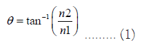
Where, n1 and n2 are the refractive indices of the two media. For glass, the Brewster angle is approximately 56.3°. This is exactly what we will use to measure the polarization of light (Figure 1) [2].

Figure 1: Illustration of the Brewster angle.
Reflection and refraction
Photons possess both wave and particle properties (wave-particle duality). Let’s examine some particle properties such as reflection and refraction.
Reflection: Reflection is the throwing back by a surface without absorbing it. The best way to get light reflections is mirrors. Given a mirror place at an angle of θm and light at an angle of incident θi, the angle of reflection can be calculated using the formula.
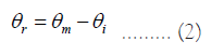
Where, θr is the angle of reflection
For example given a mirror placed at an angle of 56.3° and a light with an angle of incidence of 0 the angle of reflection will be 56.3° [3].
Refraction: Refraction is a property that refractive materials have like glass and water where particles become deflected with a different angle through the interface between one medium and another the angle of refraction can be calculated using Snell’s law.
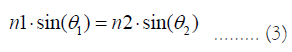
Where, n1 and n2 are the refractive indices for the two media and θ1 is the angle of incident and θ2 is the angle of refraction.
The science behind CDs as half wave plates
When it comes to the interaction of light with materials, certain objects, like Compact Discs (CDs) have interesting optical properties. One of these properties is their ability to function as half-wave plates, which can manipulate the polarization of light. To understand this phenomenon, we can delve into the principles of wave optics.
Half wave plates: Polarization refers to the orientation of the oscillation of light waves as we mentioned above. When light interacts with a surface or material, its polarization state can change. Half-wave plates are optical devices that can modify the polarization of incident light (Figure 2).

Figure 2: How a half wave plate works.
When light enter a half-wave plate, it splits into two perpendicular components: One travels along the fast axis and another along the slow axis when this two components combine again, the phase difference between them will be half a wavelength and the polarization direction will rotate by angle θnew and i can be calculated by
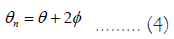
Where θ is the current polarization direction and ϕ is the angle the half-wave plate is rotated with. But half wave plates are so expensive which lead us to our next point [4].
Birefringence: Birefringence occurs because the microscopic grooves on the surface material creates two distinct paths for the polarized components of light. One component is delayed relative to the other, resulting in a something called phase shift [5]. As a result of birefringence, a CD can effectively function as a half-wave plate. This capability allows it to convert incident linearly polarized light into light with a polarization direction corresponding to that of the CD. It’s noteworthy that we can freely rotate the CD over a 360° angle.
Applications: The ability of CDs to act as half-wave plates has practical applications, especially in optical experiments and devices where polarization control is essential. Researchers and hobbyists can use CDs as cost-effective tools for manipulating polarized light and that’s exactly what we’ll be using.
Two photon interference
In order to implement 2 qubit gates we had to achieve a phenomenon called 2-photon interference. This phenomenon is an important step to enable quantum operations. We can achieve this by using the Hong-Ou-Mandel effect.
The Hong-Ou Mandel effect: This effect is a quantum interference phenomenon that arise when 2 photons are incident upon a beamsplitter. This effect result in the photons becoming entangled in such a way that they exit the beam-splitter entangled [6]. Now we can apply quantum optical gates like a half wave plate for the photons after they exit the beam-splitter by this way we can get multi-qubit gates. These gates play an important role in the manipulation and processing of quantum information so we can fully harness the potential of quantum computing (Figure 3).

Figure 3: The Hong-Ou Mandel effect.
Maths and simulations
Prior to constructing the physical hardware, one essential step was to keep track of the mathematics involved and do some simulations to validate the functionality of the hardware. As a result, we embarked on a comprehensive study of the mathematics and developed our Python library for simulating optical hardware.
Light as vectors
We started by representing the light beam as 1 × 8 vector where each element represents both the direction and polarization of the light. The vector is structured as follows, with ’H’ indicating horizontal polarization and ‘V’ indicating vertical polarization:
[RightH, RightV, LeftH, LeftV, UpH, UpV, DownH, DownV]
Optical elements as matrices
For optical elements such as beam-splitters or half-wave plates, they are represented by an 8 × 8 matrix, which we will discussing further in the code. Operations are performed by multiplying the current state with the optical matrix.
The research: After conducting some research in an effort to make
the optical element matrices as precise as possible, we arrived at
a solution utilizing trigonometric functions for amplitude and
Euler’s number for phase. Resulting in an expression that looks
like this: cos 
Optical elements examples: For example this is the matrix
representing the half wave plate in Python since the half wave
plate have a phase shift of  which is -1 so required values will be
multiplied by -1 (Listing 1).
which is -1 so required values will be
multiplied by -1 (Listing 1).
Listing 1: Code for simulating half-wave plate.
def HWP(self, theta):
theta = math.radians(theta)
first = math.cos(theta)**2 - math.sin(theta)**2
second = 2 * math.cos(theta) * math.sin(theta)
third = math.sin(theta)**2 - math.cos(theta)**2
fourth = 2 * (-math.sin(theta)) * math.cos(theta)
self.hwpmatrix = np.array([
[first, second, 0, 0, 0, 0, 0, 0],
[second, third, 0, 0, 0, 0, 0, 0],
[0, 0, third, fourth, 0, 0, 0, 0],
[0, 0, fourth, third, 0, 0, 0, 0],
[0, 0, 0, 0, first, fourth, 0, 0],
[0, 0, 0, 0, fourth, third, 0, 0],
[0, 0, 0, 0, 0, 0, third, second],
[0, 0, 0, 0, 0, 0, second, first]
])
result = self.multiply(self.state, self.hwpmatrix)
return result
Simulations
To perform simulations, we require classical computers. We chose Python as our preferred programming language and created a class called PhotonicCircuit(). This class starts with an initial state of |Right H> (which can be changed). As of now, this class can simulate four optical elements: Mirrors, beam splitters, polarizing beam splitters, and half-wave plates. We are actively exploring opportunities to expand its capabilities further. After performing simulations, you can obtain counts from the circuit. Additionally, after some careful consideration, we found out a method to measure the Z expectation value [7].
Testing: We conducted tests on simple algorithms and protocols such as the Deutsch-Jozsa or the BB84 protocol using 1 and 2-bit strings. The simulations were successful. You can access the tutorials and documentation via the following Link (https://github.com/QVLabs/WavePlate/tree/main/Tutorials).
Quantum layer simulation
Back to our main mission (a quantum layer for our neural network) we used half wave plates to get the trainable parameters and a polarizing beam splitter to get measurements notably, we opted not to use beam-splitters due to the fact that this is a 1-qubit quantum device, which we intend to expand later on the paper.
We used the parameter-shift rule to calculate our gradients [8,9]:
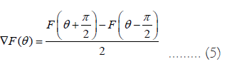
Analytic gradients Formula (https://learn.qiskit.org/course/machine-learning/training-quantum-circuits - training-19-0) and to calculate the loss we used 2 loss function for the 1 and 2 qubit devices respectively [10]
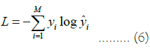
The NLL loss where ˆy is the probability distribution and y is the target
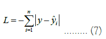
The L1 loss also known as Absolute Error You can fine all loss functions h and the quantum parameters are updated by:
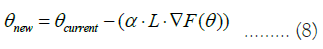
Where α is the learning rate, L is the loss, ∇F(θ) is the gradients
Final simulation result: By adding the quantum layer to our classical neural network which we will mention below the training process proceeded successfully. Full tutorial is here: (https://github.com/QVLabs/WavePlate)
Hardware
We started by creating a scheme of the 1-qubit device. The device have to contain laser, polarizer, Half-Wave Plates (HWP), mirror, Beam-Splitter (BS) and photoresistors (Figure 4).

Figure 4: Scheme of 1-qubit device. Where the mirror is placed at an angle of 56.3° and the beam splitter at an angle of 0°. Note: 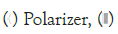

Parts of the quantum computer
We have to specify some details about all parts of the device (Figures 5 and 6).

Figure 5: Laser, polarizer and HWP.

Figure 6: Mirror, beam-splitter and photoresistor.
Laser: We are using a red laser with a wavelength of 650 nm.
Polarizer: As a polarizer we used sunglasses.
Half-Wave Plate (HWP): To generate all possible rotations of rotation gates, we decided to use a transparent refractive CD as HWP and micro servos to change angle of the CD thereby altering the wavelength of photons and subsequently modifying the probabilities [11].
Mirror: It is important to use mirrors without a glass layer (because it will make unwanted interference) so we used dental mirrors.
Beam splitter: The cheapest thing that gives the closest result to a non-polarizing beam-splitter is a piece of glass.
Photoresistor: The photoresistors were used along with a resistor of 10 k Ohm.
Arduino
To control the quantum computer we have to build two types of connections: From Classical computer to Quantum (C-to-Q) and from Quantum computer to Classical (Q-to-C). For both connections we used an Arduino.
C-to-Q: Our goal is to get the data from neural network so we can interpret input numbers as angles for rotation of HWP. To make such rotation we used Micro Servo.
Q-to-C: To get output from quantum computers we used photoresistors. We are measuring the values from the photoresistors and then counting expectation values after making measurements several times.
Required Arduino equipment: The required Arduino equipment is: Wires (mainly male-male and male-female), 2 Micro Servos, 2 photoresistors, 2 resistors (10 k Ohm) and a breadboard (Figure 7).

Figure 7: Scheme of all connections to Arduino chip.
Code for Arduino
The main loop function for Arduino takes input angles for Micro Servos from the Python NN. Then measure the values from photoresistors and then send the output back to the NN.
You can find full code here (https://github.com/QVLabs/WavePlate/tree/main/Tutorials/Actual%20Hardware/1%20Qubit/QuantumLayer) (Listing 2).
Listing 2: Code for Arduino with 2 microservos and 2 photoresistors.
void loop() {
//put your main code here, to run repeatedly:
while(Serial.available() >= 2){
for(int i = 0; i < 2, i++){
incoming[i] = Serial.read()
}
if(incoming[1] == 0){
servo1.write(incoming[0]); //qubit 0 first gate
}
else if(incoming[1] == 1){
servo2.write(incoming[0]); //qubit 0 second gate
}
}
delay(1000);
int value1 = analogRead(A0); //qubit 0 state 0
int value2 = analogRead(A1); //qubit 0 state 1
Serial.println(value1);
Serial.println(value2);
}
Building the device
To build the quantum device we used the scheme, all required parts, connected everything to the Arduino and then test it using the NN (Figure 8).

Figure 8: Upper view of the quantum device.
Neural Network (NN)
We created the Neural Network (NN) in the Python programming language that contains classical layers and the quantum layer. The dataset that we used contains pictures of ants and bees. The goal of the NN is analyse picture and say is it an ant or a bee in a given picture (Figure 9) [12].
Classical part
To create the NN we used the PyTorch library. The classical part contains 6 layers: 2 convolutional and 4 linear. Also we added a dropout function to prevent the risk of the model overfitting. In the Figure 9 you can see classical layers in the __init__ (or the main) function of the NN [7] (Listing 3).

Figure 9: Examples of data.
Listing 3: Part of the code with classical layers in the main function.
class Net(nn.Module):
def __init__(self):
super(Net, self).__init__()
super(Net, self).__init__()
self.conv1 = nn.Conv2d(3, 16, 3)
self.pool = nn.MaxPool2d(2, 2)
self.dropout1 = nn.Dropout2d(0.25)
self.conv2 = nn.Conv2d(16, 32, 3)
self.fc1 = nn.Linear(32 * 54 * 54, 1200)
self.fc2 = nn.Linear(1200, 120)
self.fc3 = nn.Linear(120, 84)
self.fc4 = nn.Linear(84, 1)
In the forward function of the NN we used ReLu as an activation function for our classical layers (Listing 4).
Listing 4: Part of the code with classical layers in the forward function.
def forward(self, x):
x = self.pool(torch.relu(self.conv1(x)))
x = self.dropout1(x)
x = self.pool(torch.relu(self.conv2(x)))
x = x.view(-1, 32 * 54 * 54)
x = torch.relu(self.fc1(x))
x = torch.relu(self.fc2(x))
x = torch.relu(self.fc3(x))
x = self.fc4(x)
Quantum part
Simulation: We created a custom layer using our own library we mentioned above, with the simulation of the actual quantum device. We implemented three functions: A function for the quantum layer, a function for getting gradients, and a function for running the circuit for gradients [13,14]. Here are the codes respectively (Listings 5-7).
Listing 5: The quantum layer.
def quantum_layer(q_input_features, q_weights_flat):
q_weights = q_weights_flat.reshape(q_depth, n_qubits).
qc = PhtotonicCircuit()
qc.HWP(22.5)
for idx, angle in enumerate(q_input_features):
qc.HWP(angle, idx)
for layer in range(q_depth):
for idx, angle in enumerate(q_weights[layer]):
qc.HWP(angle, idx)
return qc.Z_expectation(shots=20)[2]
Listing 6: Function for running the gradients.
def run(q_weights):
qc = PhtotonicCircuit()
qc.HWP(22.5)
for idx, angle in enumerate(q_weights):
qc.HWP(angle, idx)
return qc.Z_expectation(shots=20)[2]
Listing 7: Gradients function.
def apply_gradient(params):
params = params.tolist()
s = np.pi/2
gradient = []
for k in params:
k_plus = k + s
k_minus = k - s
exp_plus = run([k_plus])
exp_minus = run([k_minus])
gr = (exp_plus - exp_minus) / 2
gradient.append(gr)
return torch.tensor(gradient,dtype=torch.float32)
Actual quantum device: We created a custom layer using the serial library for sending input values to Arduino and receiving the output.
We implemented the same three functions as the simulation but with different methods to get and send data to the real quantum device (Listings 8-10).
Listing 8: Functions for sending and receiving data from the Arduino.
ser = serial.Serial(‘COM8’, 9600)
def send_to_arduino(ser, values):
ser.write(struct.pack(‘>BB’, *values))
def receive():
if ser.in_waiting > 0:
data = ser.readline().decode(‘utf-8’).rstrip()
return data
Please note that when connecting Serial, you must ensure that the Arduino is connected to the correct port. In our case, it was COM8.
Listing 9: The quantum layer with Arduino.
def quantum_layer(q_input_features, q_weights_flat):
value1,value2 = None,None
q_weights = q_weights_flat.reshape(q_depth, n_qubits)
for idx, angle in enumerate(q_input_features):
ang = angle
while ang < 0:
ang += math.pi/2
an = int(((ang*2)*180/math.pi))
send_to_arduino(ser,[an,idx])
for layer in range(q_depth):
for idx, angle in enumerate(q_weights[layer]):
ang = angle
while ang < 0:
ang += math.pi/2
an = int(((ang*2)*180/math.pi))
send_to_arduino(ser,[an,idx+1])
time.sleep(2)
while value1 == None:
value1 = receive()
while value2 == None:
value2 = receive()
print(f’value 1 is {value1} and value2 is {value2}’)
return get_exp(value1,value2)
Listing 10: Gradients function with Arduino.
def apply_gradient(input,params):
input,params = input.tolist(), params.tolist()
s = np.pi/2
gradient = []
for k in params:
k_plus = k + s
k_minus = k - s
exp_plus = run(input,[k_plus])
exp_minus = run(input,[k_minus])
gr = (exp_plus - exp_minus) / 2
gradient.append(gr)
return torch.tensor(gradient,dtype=torch.float32)
You can find the full implementation here (https://github.com/QVLabs/WavePlate/tree/main/Tutorials).
Training
Now comes the training part with used the SGD optimizer and the cross entropy loss for our training function of course after inserting the quantum layer in the neural network’s forward function (Listings 11-13).
Using the quantum layer
Listing 11: Quantum parameters in the main function in the NN where qdelta and qdepth are constants.
self.q_params = torch.nn.Parameter( q_delta * torch.randn(q_ depth,dtype=torch.float32))
Listing 12: The quantum layer in the forward function.
q_out = None
for elem in x:
# print(elem)
q_out_elem = quantum_layer(elem, self.q_params)
if q_out == None:
q_out = torch.tensor([[q_out_elem]])
else:
q_out = torch.add(q_out, torch.tensor([[q_out_elem]]))
q_out = (q_out+1)/2
q_out = torch.cat((q_out, 1-q_out), -1)
q_out = q_out.requires_grad_()
return q_out
Training the NN
Listing 13: The training loop.
network = Net()
optimizer = optim.SGD(network.parameters(), lr=0.001, momentum=0.9)
epochs = 10
criterion = nn.CrossEntropyLoss()
loss_list = []
for epoch in range(epochs):
total_loss = []
target_list = []
for data, target in dataloaders[‘train’]:
data = data.to(device)
target = target.to(device)
target_list.append(target.item())
optimizer.zero_grad()
output = network(data)
loss = F.nll_loss(output, target)
loss.backward()
optimizer.step()
#update quantum parameters
gradient = apply_gradient(output,network.q_params)
outlist = output.tolist()[0]
out = (1-outlist[0]) if outlist[0] > outlist[1] else outlist[1]
new_params = nn.Parameter(network.q_params - (0.001 * (outtarget.item()) * gradient))
network.q_params = new_params
total_loss.append(loss.item())
loss_list.append(sum(total_loss) / len(total_loss))
print(‘Loss = {:.2f} after epoch #{:2d}’.format(loss_list[-1], epoch + 1))
After completing the training, you will observe continuous improvement in the loss function. This concludes the discussion of the neural network.
Link for the full simulation tutorial here (https://github.com/QVLabs/WavePlate/blob/main/Tutorials/QuantumLayer_ Simulation.ipynb), and Hardware tutorial here (https://github.com/QVLabs/WavePlate/tree/main/Tutorials/Actual%20Hardware/1%20Qubit/QuantumLayer).
The two-qubits quantum device
We also implemented the 2-qubits quantum device so we can use entangling gates and explore other projects as well as enhance the quality of the quantum layer of our NN.
The scheme of the device
We also started by drawing a scheme of what the device should look like Figure 10.

Figure 10: The scheme of the 2 qubit device, where first beam-splitters
are placed at an angle of 45°, 90°, 0° respectively and the mirrors are
placed at an angle of 56.3°. Note: Note: 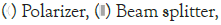

The simulation
We implemented a code using our library to simulate the scheme we designed. In this code, we developed a quantum layer that accepts input features and weights and returns the expectation value.
Link for the 2 qubit simulation tutorials here (https://github.com/QVLabs/WavePlate/tree/main/Tutorials) (Listing 14).
Listing 14: 2 qubit device quantum layer simulation.
import numpy as np
VS=[‘|RH>’, ‘|RV>’, ‘|UH>’, ‘|UV>’, ‘|LH>’, ‘|LV>’, ‘|DH>’, ‘|DV>’]
n_qubits, n_layers = 2, 1
weights = np.random.random([n_layers, n_qubits])
def 2qubitlayer(inputs, weights):
qc = PhotonicCircuit()
qc.BS(135)
# H layers
for i in range(n_qubits):
qc.HWP(22.5, i)
# INPUT features
for idx, i in enumerate(inputs):
qc.HWP(math.degrees(i), idx)
# WEIGHTS
for _ in range(n_layers):
for idx, i in weights:
qc.HWP(math.degrees(i), idx)
#--CNOT--
for i in range(n_qubits):
if i % 2 == 0:
probs = qc.measure_probs()
try:
if VS[(2**i) - 1] in probs and VS[2**i] in probs:
qc.HWP(22.5, i + 1)
elif probs[VS[2**i]] >= 50:
qc.HWP(45, i + 1)
except: pass
return qc.Z_expectation(shot=100)
You can find the full tutorial here (https://github.com/QVLabs/WavePlate/blob/main/Tutorials/QuantumLayer_ Simulation_2qubits.ipynb).
The actual hardware
CNot implementation: We used conditional operations based on the polarization properties of photons to implement the CNot gate in the simulation. Details about how this is achieved can be found in the code above. In essence, we measure the control qubit and, based on that measurement, adjust the orientation of the half-wave plate on the target qubit before measuring the target qubit.
You’ll find the Python and Arduino code here (https://github.com/QVLabs/WavePlate).
Connections: For the 2-qubit device, we used 4 micro servo motors, 4 photo-resistors and 4 10Kohm resistors for measurements, a PCA9685 chip to power and optimize everything, a 9V battery, and of course, an Arduino Uno (Figure 11).

Figure 11: The Arduino connections.
Neural network with 2-qubit device
We implemented the same neural network but with a new quantum layer and expectation value function that can process the data from and to the 2-qubit device (Figure 12).

Figure 12: The 2 qubit device.
It’s noteworthy that we replace the NLL loss with the L1 loss in the 2 qubit device.
Code: Here is the code of quantum layer with 2 qubits (Listings 15 and 16).
Listing 15: Python code for Quantum layer.
def quantum_layer(q_input_features, q_weights_flat):
value1, value2, value3,value4 = None, None,None,None
q_weights = q_weights_flat.reshape(q_depth, n_qubits)
for idx, angle in enumerate(q_input_features):
ang = angle.item()
while ang < 0:
ang += math.pi/2
an = int(math.degrees(ang))
#print(an)
send_to_arduino(ser,[an,idx])
for layer in range(q_depth):
for idx, angle in enumerate(q_weights[layer]):
ang = angle.item()
while ang < 0:
ang += math.pi/2
an = int(math.degrees(ang))
#print(an)
send_to_arduino(ser,[an,idx+2])
#time.sleep(1)
#print(‘Started layer’)
while value1 == None:
try: value1 = int(receive())
except: pass
while value2 == None:
try: value2 = int(receive())
except: pass
while value3 == None:
try: value3 = int(receive())
except: pass
while value4 == None:
try: value4 = int(receive())
except: pass {value3} and {value4}’)
return get_exp(value1,value2,value3,value4)
And this is main loop function for Arduino:
Listing 16: Code for Arduino with 4 micro servos and 4 photoresistors.
void loop() {
while(Serial.available() >= 2){
for(int i = 0; i < 2, i++){
incoming[i] = Serial.read()
}
if(incoming[1] == 0){
servo1.write(incoming[0]); //qubit 0 first gate
}
else if(incoming[1] == 1){
servo3.write(incoming[0]); //qubit 1 first gate
}
else if(incoming[1] == 2){
servo2.write(incoming[0]); //qubit 0 second gate
}
else if(incoming[1] == 2){
servo4.write(incoming[0]); //qubit 1 second gate
}
}
delay(1000);
int value1 = analogRead(A0); // qubit 0 state 0
int value2 = analogRead(A1); // qubit 0 state 1
int value3 = analogRead(A2); // qubit 1 state 0
int value4 = analogRead(A3); // qubit 1 state 1
Serial.println(value1);
Serial.println(value2);
Serial.println(value3);
Serial.println(value4);
}
You can find the full tutorial code for the 2 qubit device here (https://github.com/QVLabs/WavePlate/tree/main/Tutorials/Actual Hardware/2Qubit/QuantumLayer).
We trained the neural network and after 40 epochs we got such results: AS you can see the Neural Network started with a loss of 0.78 and ended the training with a loss of 0.067 after 40 epochs which is 30% better compared to the 1 qubit device, and using the testing dataset the NN got 148 samples correct out of 153 which gives an accuracy 96.7% (Figures 13 and 14).

Figure 13: Loss for every epoch and accuracy of the neural network for the 2 qubit device.

Figure 14: Different VLT window firm’s illustration.
By running the neural network with the 1 qubit and 2 qubit devices we have made some conclusions:
• The mean value of the loss for the 1 qubit device is -0.42, the highest value is -0.70 and the lowest value is -0.21.
• The mean value of the loss for the 2 qubit device is 0.39, the highest value is 0.78 and the lowest value is 0.067.
• There is a clear pattern that the loss exponentially go down while maintaining the same number of epochs by increasing the number of qubits.
• By training the same NN without the quantum layer with the same number of epochs we noticed a significant difference in the final performance.
• In order to get the best results from the photo-resistors the quantum computer had to operate at a total dark room.
• The simulation and math has shown that the device is fully capable of other quantum projects as well.
• There is an optical implementation for almost every quantum gate, which will enable the quantum computer to achieve its full potential.
• By increasing the quality of the components and getting new ones we can achieve much better results.
• For this moment the speed of the quantum layer is not high because of the C-to-Q connection.
• Devices similar to those can be differently interpreted. The example of this is shown in this article. We used the same dataset for both cases and the outputs supposed to give the answer (an ant or a bee). With 1 qubit device probabilities of getting 0 or 1 were used and with 2 qubit device expectation values were used.
The total cost of the 1 quit device is around 50 dollars and the 2 qubit one is around 65 dollars what is very cheap compared to other quantum computers.
The Future of the project and further devices
The project has many prospects.
• One of them is find a faster way of C-to-Q and Q-to-C connections.
• We can find a pattern in the increase of the number of qubits and their entanglement.
• We can find ways to overcome the limitations we currently have like in gates implementation for example.
• In the near future we plan to make a device with 3-4 qubits and in the future 7 and 8 qubits.
• We plan to try out different entanglement methods like the nonlinear sign-shift gate.
• Also we have ideas and plans to achieve and try more projects with the quantum devices by getting new components like a precise 50:50 and a polarizing beam-splitter, etc. and improving the quality of the exiting ones.
• In order to get a better 50:50 beam splitter we can use a window tint on the glass that has a 50% Visible Light Transmission (VLT) so we can get more better results.
• Moreover, the price of such a device will be hundreds of times cheaper than modern quantum devices, which will be perfect for learning and processing purposes.
• Also, by receiving financial support and collaborating with universities, we can improve the quality of the quantum computer accordingly, increase the accuracy of calculations.
• It is likely that in the future it will be possible to create a device with 15 qubits, the computing power of which, in theory, will be equal to the computing power of a classical computer.
Citation: Farag P (2023) Custom Quantum Devices and their Use in a Neural Network at a Quantum Level. J Phys Chem Biophys. 14:369.
Received: 16-Nov-2023, Manuscript No. JPCB-23-28037; Editor assigned: 20-Nov-2023, Pre QC No. JPCB-23-28037 (PQ); Reviewed: 04-Dec-2023, QC No. JPCB-23-28037; Revised: 11-Dec-2023, Manuscript No. JPCB-23-28037 (R); Published: 18-Dec-2023 , DOI: 10.35248/2161-0398.23.14.369
Copyright: © 2023 Farag P. This is an open-access article distributed under the terms of the Creative Commons Attribution License, which permits unrestricted use, distribution, and reproduction in any medium, provided the original author and source are credited.