Journal of Clinical and Experimental Ophthalmology
Open Access
ISSN: 2155-9570
ISSN: 2155-9570
Research Article - (2018) Volume 9, Issue 4
Keywords: Optical coherence tomography; Image processing; Automatic segmentation; CME
Macular edema and cystoid macular edema (CME) are principal causes of severe central vision loss [1]. They may appear in the retina because of several ocular pathologies [2] such as ocular inflammation, uveitis [3], retinal vein occlusion, diabetic retinopathy [4], and agerelated macular edema (AMD) [5] or after intraocular surgery [2].
Presence of single or multiple intra-retinal fluid regions (cysts) that have different sizes and forms characterize it.
Optical Coherence Tomography (OCT) is a noninvasive high resolution imaging technique allowing identification of pathologic retinal changes, evaluation of disease severity and treatment efficiency. It uses a low coherence light [6] to produce a cross sectional image of the optical reflectance proprieties of the retinal tissue [7]. It is widely used in ophthalmology for the evaluation of several ocular diseases [8-10] and has allowed a detailed description of cystoid macular edema [11,12]. CME appears in OCT images as areas of low reflectivity in the sensorineural retina [13] caused by fluid accumulation.
Current clinical practice assessment of ocular diseases with CME in OCT images is based on the measurement of retinal thickness due to its large autocorrelation with visual acuity [14-16]. However, it is proved that CME can exist in different macular disorders with absence of retinal thickening [17,18]. In addition, the retinal thickness measurement may be wrong if a sub-retinal fluid is present [19]. In another hand, there are research results, which reveal that the visual acuity may be better predicted by the retinal tissue volume than central retinal thickness in-patient with CME [20]. Actually software used on most commercial OCT-apparatus detects the retinal boundaries and gives the total macula thickness but without any quantitative information about pathologic features (such as the number and size of cystoids). Thus, quantification of the volume of fluid regions can be an important additional element for useful diagnostic metric. To calculate the total fluid volume from OCT images, automated technique of segmentation is required since it is difficult and time consuming to manually segment large 3D data. In this paper, we present an automated technique to segment cystoid regions into 3-D image stack obtained from a Spectrally OCT system (Heidelberg Engineering) and then calculate the fluid fractional volume.
As OCT is widely used in ophthalmology, the denoising and segmentation of OCT images is an active area of research. The denoising must be realized to minimize the effects of speckle noise, this latter reduces contrast in OCT image and makes the interpretation of morphological features more difficult to reach [21].
Several different techniques have been proposed to remove speckle from OCT image such as the digital filtering [21], median filtering [22,23], curvelet shrinkage [24], wavelet filtering [25,26], general Bayesian estimation [27], bilateral filtering [28-30] and anisotropic diffusion filtering [31,32]. In this study, anisotropic diffusion filtering and median filtering are used to mitigate the effects of speckle. These techniques especially succeed in smoothing noise while respecting the region boundaries and small structures, which is very important in our work.
Many methods for automatic retinal layer segmentation have been proposed to detect different numbers retinal layers. In particular, two boundaries (top and bottom layers of retina) were found by Huang et al. [6], Koozekanani et al. [33] and Ding et al. [34], three layers were detected by Baroni et al. [35], four layers were located by Shahidi et al. [36], five layers by Chan et al. [37], seven layers by Chiu et al. [38], eight layers by Ghorbel et al. [39] and eleven layers by Quellec et al. [40].
Other research works concerning fluid regions segmentation in OCT images have reported about how to delimit and quantify fluid regions existing in the retina. First, there were works, which proposed semi-automatic detection based on a deformable model initialized manually [41]. Then, many automated methods were proposed: A Knearest neighbor (K-NN) classification and graph-cut segmentation were combined [42], split Bregman technique was used as reported by Ding et al. [34], watershed was also applied by Gonzalez et al. [43] and segmentation based on thresholding with empirical parameter adjustment was implemented by Mimouni et al. [1] and Wilkins et al. [29]. Recently, a machine learning approach with an effective segmentation framework based on geodesic graph cut was proposed by Bogunovic et al. [44], a random forest classifier was used to classify the microcystic macular edema by Lang et al. [45], a kernel regression (KR)-based classification method was developed to estimate fluid and retinal layer positions by Chiu et al. [46] and an automated volumetric segmentation algorithm based on fuzzy level-set method was presented by Wang et al. [47]. Also, a retinal cyst segmentation challenge was hosted at the MICCAI 2015 conference in which several novel cyst segmentation techniques were developed using different methods [48-52].
The previous methods using thresholding yield good segmentation [1,29]. However, the thresholding values used were empirical fixed by the authors for all B-scan images acquired from different patient. In this work, a fully automatic process for intraregional fluid segmentation using automatic thresholding calculation is described. It calculates the thresholding value automatically for each patient volume, identifies fluid regions in a retinal volume stack and then fluid is quantified. The presented method contains three basic steps namely, a preprocessing one, the layer’s segmentation step and the regions segmentation step.
Data acquisition
The Spectrally device (Heidelberg Engineering, Heidelberg, Germany) was used to obtain OCT images. OCT-images used in this study were acquired from 2 normal patients and 8 patients with vitreoretinal disorders and evidence of intra-retinal cysts.
Of the ten subjects used in our study (2 healthy subjects and 8 pathological suspects), about 100 images were collected per OCT technique for each case.
Our method of segmentation of the intra-retinal fluid is applied to all these images constituting our database (more than 1000 images) and the results that are exposed in this paper is in fact an average image in each studied case.
The OCT volumes data contains 19 B-scans (the 2 normal patients), 25 B-scans (1 patient) and 49 B-scans (7 patients) with varying image quality. Each volume comprised a 6 mm × 6 mm × 1.8 mm data cube. Averaging of the B-scans was determined by the acquisition device, and ranged from 8 to 25 raw images per averaged B-scan. Every B-scan image contains 512 × 496 pixels with axial and lateral resolution of 3.8 μm and 14 μm, respectively. The B-scan images are spatially distinct, they do not overlap, so they were segmented and processed independently (Figure 1).

Figure 1: Input SD-OCT scan.
We can specify that these automatic methods wouldn’t work on images acquired from other OCT technologies than Spectrally OCT (Heidelberg Engineering).
The main purpose of this study in this paper is to quantify the volume of retinal fluid to diagnosis and screening the Macular edema and cystoid macular edema (CME) pathology.
The other methods of retinal imaging such as the Heidelberg Retina Tomography (HRT) who is based on fast and reproducible topographic measurements or SLO (Scanning Laser Ophthalmoscope) one would have obtained 2D-fundus retinal images where it is difficult to calculate the volume of retinal fluid because the OCT acquisition method provides retinal slices images where it is better to specify the volume of fluid opposing to other image profiles of the retina where it is easier to segment the edge of the optic nerve head ONH and not the volume of the retina fluid.
The SLO is based on scanning a laser brush on the retina. The return signal makes it possible to reconstruct the observed field and thus to establish an accurate mapping of the retinal surface, with the topographical references, even in the presence of alteration of the transparency of the media. OCT is comparable to ultrasound (although based on light, not ultrasound) and allows visualization of organ "slices" (less than 10 microns thick) by penetrating tissue depth.
With this technology, optical retinal sections are obtained with a separating power of about 5 microns in axial section and 15 microns in transverse section for the most advanced versions (let us recall for information that the length of the outer article of a stick varies from 30 to 50 μm).
Thus, thanks to the joint use of both techniques, the operator can choose the location of the retinal section (vessels, optical disc or area central retina for example).
Remember that SLO/OCT imaging is a complementary examination that must naturally be part of a reasoned clinical approach.
Degenerative disorders: whatever the etiology, any degenerative affection results in the thinning of the layer of the cells concerned; in the context of a recent modification of the visual behavior of a suspect and when the electroretinography signs are not yet interpretable, the OCT may allow an early etiological diagnosis.
The proposed method consists of three steps, preprocessing step, layer segmentation and fluid region segmentation (Figure 2).

Figure 2: Flowchart of the proposed algorithm.
In pre-processing step, OCT scans are initially denoised by using median filter for layer’s segmentation and anisotropic filter for region segmentation. Then the B-scan images are segmented. During retinal layer segmentation, the top and bottom layers of retina are detected. The positions of these layers are used in region segmentation, to define the retinal ROI in each B-scan image. Potential cystoids fluid area is defined through contiguous pixel regions within the retinal ROI. The value of thresholding is automatically calculated.
Retinal layer segmentation
To define the retinal ROI region, internal limiting membrane (ILM) (the top retinal layer) and retinal pigment epithelium (RPE) (the bottom retinal layer) need to be segmented.
In pre-processing step, the OCT scans are first denoised using the median filter [23,24,37] . It was used over 3 × 3 pixels in x × z directions. Then, two processes are performed the first to detect the ILM and the second to find the RPE layer.
Detection of the internal limiting membrane (ILM)
The internal limiting membrane is the boundary between the retina and the vitreous. It’s a highly reflective layer because of the high difference in the refraction index, between vitreous and retina. Five sequential steps were applied in the segmentation process as shown in Figure 3.

Figure 3: Flowchart of the proposed segmentation method of the ILM.
After pre-processing, a K-means classification (k=2 classes) is applied to the B-scan image (Figure 4).

Figure 4: Results of the applying of the K-means classification to the B-scan image
The vitreous pixels are classified in class 1 (dark regions), while the pixels of the retina are classified in class 2 (white color). A customized Canny Edge detector, which is recognized as a well-optimized edge detector [53], is used. Since the ILM layer has a high contrast, a high threshold is set to detect this boundary and remove vitreous noise classified as white pixels by the K-means classifier (Figure 5 (the noise is marked by the arrows) and Figure 6-d).
Figure 5: Detection of the boundary and remove vitreous noise classified as white pixels by the K-means classifier.

Figure 6: (a) Original image acquired with the Spectralis device (b) Result of the median filter (c) k-means segmentation (label 1 in black, label 2 in white) (the arrows marks the noise classified; (d) Result of Canny edge detector (e) Final ILM segmentation. (f) The reference ILM image created from the stored coordinates.
The next step aims to localize the ILM. The Canny edge output image is binary as shown in Figure 6-d, the boundaries are in white. Since, the ILM is the first white boundary from the top, a pixel (x0, z0) is selected as the first white pixel of a scan from top to bottom applied on the central column  Starting from the picked pixel (x0, z0), the ILM layer is iteratively detected, column by column, by finding the white pixels in the column and choosing the closest to the previously ILM founded pixel. Coordinates of found pixels are saved in two different vectors; one for the lines and the other for columns. Finally, a reference ILM image is created from the stored coordinates as shown in Figure 3-f.
Detection of the retinal pigment epithelium (RPE) layer
The retinal pigment epithelium (RPE) appears as a high intensity layer above the choroid (Figure 7-a). Inspired by the work proposed by Ghorbel et al. [39], a technique based on searching the maximum intensity level along each A-scan profile in the B-scan image is applied.

Figure 7: (a) A-scan profile: red curve before filtering and blue curve after filtering. (b) Final RPE segmentation result.
The segmentation is proceeded in three steps; first a median filtering is applied to the B-scan image. Then, each A-scan on the image is filtered using a low-pass filter handled by a digital filter based on a rational transfer function in the Z-transform domain [54]. Finally, the outside of RPE is detected, column by column, as the maximum on each column in the filtered image.
The coordinates of found pixels are saved in two different vectors; one for the lines and the other for columns. Finally, a reference RPE image is created from the stored coordinates as shown in Figure 7-b.
Retinal ROI image
The images of references obtained from the ILM segmentation and the RPE segmentation are used to create the retinal ROI image as shown in Figure 8.

Figure 8: Retinal ROI image.
Intra-retinal fluid segmentation
First, anisotropic diffusion filter [55] is applied to denoise each OCT B-scan image. This technique of filtering has shown a good performance in terms of reducing speckle noise and edge preservation in OCT images by Quellec et al. [40] and Garwin et al. [56]. Then, the B-scan images are segmented using an automatic thresholding [57]. The used thresholding technique is based on automatic selection of an optimal gray-level threshold value to separate objects of interest (the intra-retinal fluid) in a B-scan image from the background (the retina) by using their gray-level distribution. The proceeding algorithm is as follows:
1. For each B-scan image in the stack of images:
- Step 1: Create a histogram of the image pixel intensities
- Step 2: Detect the peaks which have the maximums heights in the histogram (Figure 9-(a))

Figure 9: (a) Histogram of B-scan image. (b) B-scan image after thresholding. (c) The automatic segmentation result. Note: b) The black pixels present the detected fluid and white pixels present the background.
- Step 3: Find the gray level values of detected peaks. This produces two gray level values; V1 the gray level value of the first peak and V2 the grey level value of the second peak
- Step 4: Calculate the local threshold value as the mean value of V1 and V2.
- Step 5: Save the local threshold value computed from each B-scan image.
2. Compute the global threshold value S as the mean of saved local threshold values.
3. Segment each B-scan image in the stack of images using S. This produces two groups of pixels. G1 consisting of all pixels with gray level values >S and G2 consisting of pixels with values <=S.
4. Extract the pixels corresponding to the intra-retinal fluid as they obey to these two conditions:
- Condition 1: The pixel belongs to G2 (G2 consisting of pixels with values <=S).
- Condition 2: The coordinates of the pixel are located between the ILM and the RPE in the ROI reconstructed image.
Quantification of the intra-retinal fluid
The above algorithm was applied for all B-scan images on each stack of images. The output layers’ segmentation and the output fluid segmentation are used to calculate the fluid and retinal tissue area from the B-scan images. The function A(In) of segmented areas in each B-scan image was obtained, for n=1, 2, 3, …, N where N is the number of images in the studied stack of images. To compute the total intraretinal fluid volume Vf, the function A was numerically integrated as in the following equation:
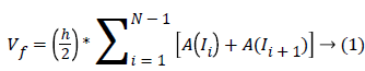 Where h is the distance between the B-scan images
To assess the performance of the proposed automatic segmentation, the technique was applied on a dataset of 10 OCT volumes from 10 subjects: two healthy control subjects and 8 subjects diagnosed with macular edema associated to diverse retinopathy.
To constitute the ground truth, two clinical experts (i.e., ophthalmologists) manually segmented all OCT B-scan images. The ophthalmologists are asked to trace the intra-retinal fluid contours using a computer mouse in a specific algorithm permitting to trace and extract the fluids on each B-scan image in the experimental datasets. Due to the time consumption of manual segmentation for each volume data, 6 volumes data are totally segmented and the two other volumes were partially segmented (13 out of the 49 B-scans). The selected Bscan images used in the partial datasets are centered on fovea scan (fovea scan ± 6).
To evaluate the proposed method accuracy, the results of the automatic segmentation are compared to manual segmentation performed by the Expert 1 (E1) and Expert 2 (E2). The precision, the specificity, the false positive rate (FPR) and the dice similarity coefficient (DSC) measures as presented by Shi et al. [30], Nguyen et al. [58], Gasparini et al. [59] and Udupa et al. [60] are calculated as follows:
Precision=TP/(FP+TP)---(2)
Specificity=TN/(TN+FP)---(3)
FPR=FP/(FP+TN)---(4)
DSC=2|TP|/(2|TP|+|FP|+|FN|)---(5)
With TP: True positives, FP: false positives, TN: true negatives and FN: false negatives [61]. The detection method is considered efficient if the precision, DSC and specificity are high and the FPF is low [59].
Figure 10 shows the qualitative results of automatic segmentation algorithm comparing to manual segmentation for varying amounts of edema including case where there no visible fluid available (Figure 10 (c), (f) and (i)). The algorithm was able to detect most fluids regions. The general visual inspection, of obtained images by the proposed segmentation, yield to visually acceptable fluid regions extraction approving quantitative information about fluid in appropriate form.

Figure 10: Qualitative results for the segmentation of fluid on SDOCT B-scan images of eyes with different amount of edema. (a-c) Original images with significant, moderate and no visible fluid, respectively, (d-f) their corresponding manual segmentation, (g-i) the automatic fluid segmentation. Note: (d-i) the black pixels present the detected fluid and white pixels present the background.
The total retinal volumes, the total volumes occupied by the fluid on the proposed segmentation and on the experts’ segmentations (E1 and E2 separately) are calculated. The precision, specificity, FPR and DSC compared to performance of expert 1 (E1) and expert 2 (E2) are reported in Tables 1 and 2, respectively. Note that, the subjects 1 and 2 highlighted in the tables are healthy. Subscripts 1 and 2 were added to the performance values to differentiate the values related to expert 1 from the values related to expert 2.
| Subject index | # of images in stack | Precision1 (%) | Specificity1 (%) | FPR1 (%) | DSC1 (%) | Retinal volume (mm3) | Measured Fluid % volume | Expert 1 Measured Fluid % Volume |
|---|---|---|---|---|---|---|---|---|
| Subject 1 | 19 | Control | 99.83 | 0.17 | Control | 9.7 | 0.03% | 0% |
| Subject 2 | 19 | Control | 99.97 | 0.028 | Control | 8.75 | 0.09% | 0% |
| Subject 3 | 49 | 90.75 | 99.99 | 0.005 | 93.62 | 8.93 | 0.95% | 1.33% |
| Subject 4 | 49 | 91.4 | 99.96 | 0.041 | 92.27 | 9.66 | 1.97% | 1.97% |
| Subject 5 | 49 | 63.94 | 99.84 | 0.16 | 64.28 | 12.38 | 1.84% | 1.63% |
| Subject 6 | 25 | 67.56 | 99.99 | 0.01 | 60.23 | 9.9 | 0.32% | 0.33% |
| Subject 7 | 49 | 81.89 | 99.13 | 0.87 | 85.49 | 15.46 | 25.96% | 30.44% |
| Subject 8 | 49 | 73 | 99.84 | 0.16 | 70.97 | 12.23 | 3.98% | 1.46% |
| Subject 9 | 13 | 95.59 | 99.93 | 0.074 | 93.78 | 2.69 | 8.35% | 8.63% |
| Subject 10 | 13 | 91.79 | 99.94 | 0.06 | 93.65 | 2.39 | 4.10% | 3.93% |
| Mean | -- | 81.99 | 99.82 | 0.171 | 82.22 | -- | 5.93% | 6.22% |
| Median | -- | 86.32 | 99.93 | 0.067 | 89.33 | -- | 2.97% | 1.80% |
| Std. Dev | -- | 12.31 | 0.28 | 0.288 | 14 | -- | 8.48% | 10.13% |
Table 1: Comparison of quantitative measures from proposed segmentation and expert 1 segmentation.
| Subject index | # of images in stack | Precision2 (%) | Specificity2 (%) | FPR2 (%) | DSC2 (%) | Retinal volume (mm3) | Measured Fluid % volume | Expert 2 Measured Fluid % Volume |
|---|---|---|---|---|---|---|---|---|
| Subject 1 | 19 | Control | 99.83 | 0.17 | Control | 9.7 | 0.03% | 0% |
| Subject 2 | 19 | Control | 99.97 | 0.028 | Control | 8.75 | 0.09% | 0% |
| Subject 3 | 49 | 95.04 | 99.99 | 0.005 | 87.81 | 8.93 | 0.95% | 0.93% |
| Subject 4 | 49 | 92 | 99.96 | 0.038 | 91.8 | 9.66 | 1.97% | 2.99% |
| Subject 5 | 49 | 79.3 | 99.9 | 0.091 | 69.21 | 12.38 | 1.84% | 2.38% |
| Subject 6 | 25 | 63.26 | 99.99 | 0.013 | 49.66 | 9.9 | 0.32% | 0.29% |
| Subject 7 | 49 | 86.44 | 99.34 | 0.66 | 88.4 | 15.46 | 25.96% | 32.75% |
| Subject 8 | 49 | 76 | 99.86 | 0.14 | 72.67 | 12.23 | 3.98% | 4.61% |
| Subject 9 | 13 | 96.39 | 99.4 | 0.061 | 93.3 | 2.69 | 8.35% | 8.82% |
| Subject 10 | 13 | 95.72 | 99.97 | 0.031 | 85.41 | 2.39 | 4.10% | 4.76% |
| Mean | -- | 85.51 | 99.87 | 0.13 | 79.78 | -- | 5.93% | 7.19% |
| Median | -- | 89.22 | 99.95 | 0.049 | 86.61 | -- | 2.97% | 3.80% |
| Std. Dev | -- | 11.83 | 0.21 | 0.218 | 14.96 | -- | 8.48% | 10.67% |
Table 2: Comparison of quantitative measures from proposed segmentation and expert 2 segmentation.
As displayed, compared withprecision1and specificity 1, precision 2 and specificity 2 increased slightly. The FPR2 showed an improvement compared to FPR1 whereas DSC2 decreased a little compared with DSC1. The overall mean values are comparable to the inter-manual results which yielded an averaged precision, specificity, FPR and DSC of 84.01%, 99.9%, 0.14% and 87.63% respectively.
The FPR values are due to detection of regions presenting low reflectivity such as blood vessels. In datasets used in this study, only the subject 7 (Table 2 presented a FPR >0.2% due to presence of abnormal growth of blood vessels. Notice that, the control datasets presented a mean error volume of 0.06%, which is a result of falsely detection of outer plexiform and outer nuclear layers as fluid in images having poor contrast (Figure 10-(f)).
To improve the accuracy of proposed technique, the blood vessels regions falsely detected by the algorithm may be rejected by applying a suppression process such as the method described by Wilkins et al. [29] or use the intensity and size-based criteria as proposed by Shi et al. [30].
The performances of Expert 1, Expert 2 and proposed method are compared in Figure 11 and Figure 12. Generally, the proposed method perfectly detects the large fluid regions but the performance decreased where the regions are small (Figure 11). The automatic segmentation correlated better with average volume of E1 and E2 (Figure 11(c)). As shown in Figure 11 (d) and Figure 12 (b-d), the expert 1 gave a smaller fluid volume compared to expert 2. E2 found more small fluid regions than E1 and they were larger as well (Figure 12 (b-d)).

Figure 11: Inter segmentation evaluation. Scatter plot of fluid volume between automatic segmentation and Expert 1 (a), Expert 2 (b) and the average of Expert 1 and Expert 2 (c), and the associated R-squared values. (d) Scatter plot of fluid volume between Expert 1 and Expert 2, and the associated R-squared value.

Figure 12: Comparison of automatic and expert’s segmentations. (a) Original B-scan image with severe macular edema, (b-d) Expert 1 and Expert 2 segmentation results respectively, (c) Automatic segmentation result. Note: (b-d) the black pixels present the detected fluid and white pixels present the background.
Figure 10 shows the fluid volume values obtained by the different segmentations on all subjects. Except for the first 2 subjects, the automatically obtained fluid volumes are smaller than the average volume values of expert 1 and expert 2. According to Tables 1 and 2, the average fluid fractional volume is 5.934% when calculated by the proposed segmentation, 6.215% by the clinical expert 1 and 7.194% by the clinical expert 2. The difference is due to undetected true fluid regions which are generally the small fluid regions as shown in Figure 12 (c) and Figure 12 (d).
A minimal computational time is needed to accomplish this technique. A full stack of 49 B-scan images is preceded in 90 seconds on a 64-bit PC with 4 GB of RAM and a 2.67 GHz. The retinal layer segmentation is the most consuming step (55%). To reduce the computational time, the algorithm can be implemented in a compiled programming language (Figure 13).

Figure 13: Comparison of fluid volume from the two experts and automatic algorithm.
Even several methods were proposed and largely used, overly complicated methods with a large number of finely tuned parameters may be fitted to the evaluated data and their performance may not be adequate in a clinical setting. The most advantage of the proposed method over other methods is its simplicity while maintaining good performance. Furthermore, it is rapid and not time consuming that can motivate its use in clinical routine.
In this study, the method was only tested in high-quality Spectrally images. Spectrally B-scans have typically a higher contrast and less noise than B-scans from other instruments, obtained by averaging a larger number of B-scans at the same position. To affirm that this method is an efficient tool, further validation studies are needed. However, the proposed algorithm should be applied on a large datasets images containing datasets from different vendors. Furthermore, actually the method depends on the layer segmentation results. If the layer segmentation is erroneous, it will alter the segmentation and can lead to wrong classification.
In order to provide a metric that may contribute to diagnostic of visual acuity, we presented an unsupervised method for the segmentation and quantification of total volume taken by cystoid fluid in OCT images. The results indicate that the proposed algorithm represents a reliable method of total fluid volume evaluation. The average precision, specificity, DSC and FPF are 83%, 99%, 81% and 0.15%, respectively. We found that undetected fluid regions were typically small and have a less effect on the total fluid volume estimation.
The results obtained from the comparison between the automatic and manual segmentations, are evaluated by two expert’s opinion and indicate good performance. To affirm that this method is an efficient tool, further validation studies are needed. However, the proposed algorithm should be applied on a large datasets images. In our case, false positive regions detected are minimal but it is possible to improve our method by adding a process allowing the suppression of these regions falsely detected.
Currently, this technique is fully automatic and works on images directly acquired from Spectralis OCT (Heidelberg Engineering). We expect that this technique may contribute to continuous improvement of OCT images segmentation notably related to automated thresholding of CME regions.