Journal of Clinical Trials
Open Access
ISSN: 2167-0870
ISSN: 2167-0870
Research Article - (2016) Volume 6, Issue 4
Multi-stage clinical trial, also termed group sequential clinical trial, is commonly used design for clinical trials to evaluate a new treatment against existing one(s). Such design allows the trial to stop early for pronounced treatment effect or the lack of it thereof based on data accumulated at the intermediate stage. The sequential conditional probability ratio test (SCPRT) approach is derived based on the concept of discordance probability, namely, the probability that the decision to accept or reject the null hypothesis based on interim data would reverse should the trial continue to the planned end. This probability is controlled at a preset small level. It is one of the intuitively appealing procedures along with stochastic curtailing but the procedure has been shown to be more efficient than the procedures based on stochastic curtailing. However, in the existing SCPRTs, the discordance probability, type I error and power are not easy to compute. Here we investigate a simulation based method to compute these quantities and apply them to a real data problem as an illustration.
Keywords: Conditional probability ratio test; Discordance probability; Type I error; Power; Multi-stage clinical trial; Stopping boundary
Multi-stage clinical trial is commonly used to evaluate a new treatment against some existing one(s) [1,2]. For one-stage (also called, non-sequential) clinical trial design, with a given nominal level α, the stopping boundary is the level α critical value for the test of the null hypothesis of no difference among the treatments. For multistage clinical trial designs, stopping boundaries should be designed to ensure the overall (or family-wise) type-I error be approximately at the specified level α. These boundaries serve as stopping guidelines to prevent inappropriate early stopping. Such boundaries are not unique, and there are large numbers of researches on this problem. It is now common in phase III trials sponsored by pharmaceutical industry and the National Institute of Cancer to include interim monitoring boundaries in the protocol documents [3-6].
Commonly used stopping boundaries include the O’Brein-Fleming boundary [2] and the corresponding spending function or a variant of it. The sequential conditional probability ratio test (SCPRT) boundary [7-9] is derived based on the concept of a negligible discordance probability, namely, the chance that the decision to accept or reject the null hypothesis based on interim data will reverse would be should the trial continue to the planned end. The approach is computationally more complex and once the multistage (i.e., boundary) is chosen, we can calculate the discordance probability of this design and the SCPRT boundary has the feature that it can control the discordance probability at a preset small level so that the probability that conclusion obtained at an early stage and that at the end of the trial differ is very small and negligible. The calculation of the probability is our focus here. However, in the existing SCPRT, the discordance probability, type I error and power are not easy to compute, and are only given for some selected configurations of stages, interim sample sizes and are only available for balanced design. In practice, it is desirable to compute these quantities for any given configuration of stages, interim sample sizes, balanced or imbalanced. Here we investigate a simulation method to compute these quantities for general setting of configurations. The simulation results are reported and the method is illustrated with a real data example.
In Section 2 we describe the problem and the SCPRT procedure, Section 3 describes the proposed simulation method for computing the discordance, type I error and power for the SCPRT. Section 4 presents the simulation results for some selected configurations of stages, interim sample sizes, for both balanced and imbalanced cases, and applies the method to a real data set as an illustration.
The problem and Brief Review of the SCPRT
As mentioned in the Introduction that sequential tests are commonly used in clinical trials. The SCPRT is a special such test, developed by Xiong [7], Tan, Xiong and Kutner [8], Xiong, Tan and Boyett [9], etc. With the SCPRT, if a trial is stopped early with a conclusion, then statistically the same conclusion would likely to hold had the trial continued to its planed end, so that consistent conclusions can be achieved with high chance using this sequence of tests. In clinical trial, often the parameter θ of interest is the difference among the treatments, and the goal is to test the null hypothesis H0: θ ≤ θ0 vs Ha: θ > θ0. Consider a group sequential test with k-stages, let n1 < ··· < nk be the cumulative sample sizes at these stages, set tj = nj/nk. At each stage-j, we compute a statistic Sj from observations based on the nj individuals, and make a decision whether to stop/continue the trial to the next stage, and make a conclusion about the treatment, based on Sj. Let sk0 be the cutoff value of Sk in a non-sequential trail. In SCPRT, at each stage time tj, a decision, either stopping the trial or continue to the next stage of the trial, is determined by the following conditional maximum likelihood ratio
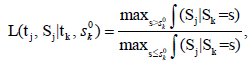
Where ∫(Sj |Sk ) is the conditional density of Sj given Sk, and it is free
of the parameter θ, as long as Sk is a sufficient statistic for θ. The decision rule is of the format: continue to the next stage if 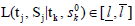 for some
  to be determined such that the test has a given nominal level α and power. In general the above conditional maximum likelihood, and hence
  and
and  are difficult to evaluate. However, if Sj is a Browning motion with drift θ on an unit time interval, i.e., Sj∼N(θtj,tj)(j=1, ..., k; tk=1), then the likelihood ratio is easy to evaluate in closed form,
  for some is equivalent to Sj∈ [aj, bj] for some −∞ < aj < bj < ∞ [9] and the boundaries [aj, bj]’s are determined such that the family wise type I error of the sequential test is under control by a given nominal level α and power. In this case, these boundaries are feasible to evaluate, and will be our focus hereafter. To be specific, if assume the responses X1, ...,Xnk iid N(μ, σ2), with σ2 known. We want to test H0: μ ≤ μ0 vs H1: μ > μ0. Under this assumption,
 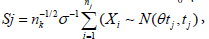 with
with 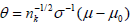 and
and  (j = 1, ...,k).In clinical trial, often the Xi’s are the differences between the new and existing treatments, and we are interested in testing the hypothesis H0: θ ≤ 0 vs Ha: θ > 0. Here θ=O(nk-½) corresponding to a local alternative, which is more reasonable than the fixed alternative.
The SCPRT stopping boundaries for the one-sided hypothesis H0 vs Ha in a k-stage clinical trial are given as
 (1)
(1)
Where tj=V ar[Sj]/V ar[Sk] is called the time information fraction. Recall that we have one-sided test, so for the non-sequential trial, when the test statistic Sk>zα, we reject H0; otherwise accept. For the sequential trial, at an intermediate stage j, if Sj∈[aj,bj]c, we stop the trial and make a decision; if Sj>bj , we reject H0; if Sj < aj , we accept H0; if Sj ∈ [aj,bj], the trial is continued to next stage. For the final stage k, ak=bk=zα, so it’s always stop. If Skbk, we reject H0, otherwise accept. In particular, if the observed data are iid, then tj=nj/nk; z is the (1-α)- th upper quantile of the standard normal distribution, and the values of a=a(k, ρ) and b=b(k, ρ) depend on the maximum conditional discordance probability ρ (or the maximum discordance probability ρmax), the number of stages k and the time points of each stage (the information times). In practice often a symmetric boundary pair is used, i.e. a=b, and with balanced information times (or tj-tj−1=1/k for j=2, ..., k). In this case the values of a=a(k, ρ)(=b =b(k, ρ)), which depends on k, ρ and the sample standard deviation σ, are given in Table 1 in Xiong, Tan and Boyett [9], for some given σ.
As an example, if the trial has k=4 stages with a known σ, and we choose ρ=0.02, then from Table 1 in Xiong, Tan and Boyett [9] we find a(= b)=2.953; if we choose ρ=0.005, then a(= b)= 4.227; and the corresponding lower/upper boundaries ar/br are obtained by (1).
Other values of a for some selected configurations of k, (n1,...,nk) and ρ are given in Table 1 of Xiong, Tan and Boyett [9]. Our goal in this communication is to present a simulation based method to compute the discordance probability, type I error and power of the SCPRT procedure in the general case.
Discordance probability
The computation of discordance probability is technical, so below we will first review some of its basic facts. In group sequential clinical trial, the decision can be made at some time point nj ahead of the planed final stage at time nk, and the decision made at time nj may differ to that made at the final time point nk if the trial were continued to the end of the trial. It is impossible to make sure that any early decision would be the same as the one made at the end of the trial should the trial went on. Intuitively, a good group sequential clinical trial should be such that the chance of difference between an early decision and that of the nonsequential trial made at the end should be small (but not too small, for one can make the stopping boundaries of the intermediate stages arbitrarily large so that there is no intermediate stop and the multi-stage trail is the same as a single stage one). The discordance probability of a multi-stage clinical trial is the probability that the sequential test and the non-sequential test lead to different decision (reject/acceptance of the null hypothesis) when both are used on the same sequence of observations. For formal definition of this concept and its computation and detailed properties we refer to the paper of Xiong, Tan, Kutner [10] and citations there.
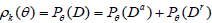
Let P(D) be the discordance probability, it is related to k and the (aj,bj)’s. Let N be the stopping time of the sequential trial, Ba and Br be the acceptance and rejection regions for (N, SN) for testing 0 H0:θ ∈Θ vs.: a Ha θ ∈ Θ . Let Ra and Rr be the acceptance and rejection regions for the same test based on the non-sequential test Sk, with nk fixed. For a sequential clinical trial with k stages, Define the events
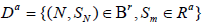 and
and 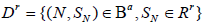
Then D = Da ∪Dr , and the discordance probability between the statistics (N, SN) with k stages and Sk is
Note also that

since P (N > nk)=0 , as nk is the final stage time point. Let
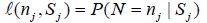
Let 1(·) be the indicator function. By Theorem 3.1 in Xiong, Tan, Kutner [10],

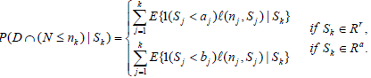 (2)
(2)
For a sequential clinical trial with k stages, the conditional discordance probability is defined as (Xiong, Tan, Kutner [10]) ρk,s=P(D|Sk=s), and by (2),
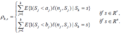 (2)
(2)
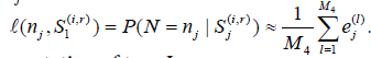
In (2) or (3), we need to compute the l(nj,Sj)'s. For continuous end points, typically the normal distribution is assumed, i.e 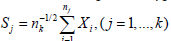 with the xi’s iid N(μ, σ2). Thus, for i < j,
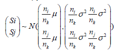
and Si | (Sj = s) ~ N(μ1 ,σ12 ) , with
 and
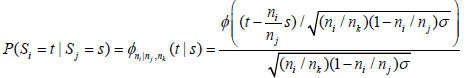
and  Thus, for i< j, P(Si = t|Sj = s) is given by
or  and the l( nj,Sj)'s can be computed via the following iterative formula
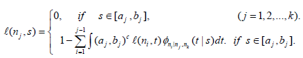 (4)
(4)
In particular  .
.
The above iterative formula for the  is not easy to use via simulation based method, as it involves multiple integration. Below we consider another expression for the also from Xiong, Tan, Kutner [10]. Let N be the stopping time, and
  Then by Theorem 2.2 and Example 2.1 in Xiong, Tan, Kutner [10],
  for s∈ [aj ,bj] and

 (5)
(5)
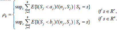
In Xiong, Tan, Kutner [10], the a =a(k,ρk)'s and b=b(k,ρk)'s are computed mainly via (3). See also Xiong [11] and Xiong and Tan [12]. For each fixed k, they find a =a(k,ρk) b=b(k,ρk) and for the maximum value of ρk,s. For this, let ρk=sups ρk,s ρk,max= sup θρk(θ), then a and b are determined by ρk or ρk,max. Note ρk)(θ) ≤ ρk,max ≤ ρk. Also, for very small (or large) values of s, any early decision and the final stage decision should agree (accept or reject), so ρk exists and should be achieved at some moderate value of s. Using ρk, a and b are determined by the equation
 (6)
(6)
However, (a, b) determined by (6) depend on k and given value of ρk. In the case of symmetric (a=b) and balanced trial (equal distance among the stage time points), Table 1 in Xiong, Tan, Boyett [9] gives values of a for different k and ρk. Even for this case, the computation is non-trivial, especially for large k. For the symmetric case, below we consider a simulation based method for the computation of a=a(k, ρk).
The Proposed Method
Assume symmetric boundary, then the stopping boundary for the j-th stage is [9],

Computation of discordance probability
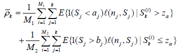
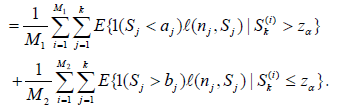
To emphasize its dependence on a, we re-write ρk in (6) as ρk(a). However, the supreme in (6) is not easy to evaluate, so we consider the expected conditional discordant probability, given by
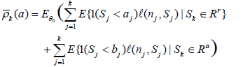
One may attempt to minimize the above expected conditional discordance probability over a (or the maximum conditional probability, or ρmax), however this does not make sense. If we take a to be sufficiently large, then at each stage time nj, Sj will always be in [aj, bj] so that there is no stopping at any intermediate stage, and the sequential trial becomes the same as the non-sequential trial, and the discordance probability is zero. This is not desired, as we want the sequential trial to be different from the non-sequential one, and has the chance of actual early stop if extreme results observed at an intermediate stage. So the values of a can only be computed with each subjectively given value of  (or ρ, or ρmax) and the values of (or ρ, or ρmax) should be chosen such that the probability of the conclusion by sequential test being reversed by the test at the planned end is small, but not too small [7,8].
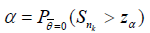
Under θ0=0, assume σ=1, 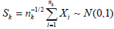 and for given level α, Ra={Sk ≤ za} with za being the (1−α)-th upper quantile of N(0, 1).
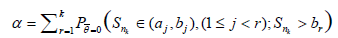
Note 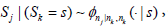 or
or 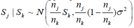


So (7) is re-written as 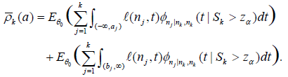 (8)
(8)
Below, for given a, we compute  (a) using (8) by simulation. We use the values of a given in Table 1 of Xiong, Tan, Boynett [9], and compute the corresponding (a) for each k = 2, ..., 10. For each given a, the computation is given via the following steps
i) Compute the right hand side of (8). The computations will involve the  the
the  and the
  )dt s.
In particular,  For j > 1 the
  are given by (5), and so we also need to compute
  .
.
For given , for i = 1, ...,M (typically M = 10, 000), sample sk(1).....sk(m) k iid N(0, 1) (under θ0 = 0), let  and
and 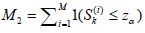 then the right hand side of (8) is computed as
 (9)
(9)
 (9)
(9)
Note in the above we only use the S(i) k ’s satisfying either the condition Sk(i) > zα or Sk(i) ≤ zα.
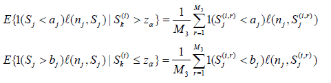
ii). In i), for each fixed j, we need to compute  (i = 1,...,M1) and
 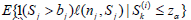 (i = 1, ...,M2). For this, for each fixed i and Sk(i) , for r = 1, ...,M3 (typically M3 ≥ 10, 000) and d = 1, 2, ..., j, sample
 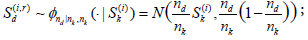 and set
iii) In the above we need to compute  for each Sj(i,r)and j = 1,...,k. For j = 1,
 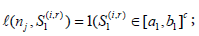 For each (j, i, r) with j > 1, for l = 1,...,M4, sample
 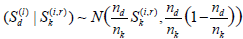 (d = 1, ..., j − 1). then count the number ej(l ) of times N(l) = nj, i.e., ejl=1 if Sdl∈ [ad bd] for d = 1, ..., j − 1 and Sjl∈ [a j bj]c ; otherwise set ejl=0. Set
Computation of type I error
Recall in the single stage case, the theoretic (or asymptotic) type I error is the significance level α, while the observed type I error for testing H0 vs H1 in the simulation is
In the general k(>1) stages case, we need to control the family-wise type I error to be no more than α, and for continuous type statistic, to be equal α i.e.,
Simulation algorithm: Denote  Given M (typically M ≥ 10,000). Set e = (e1,....,eM) = (0, ..., 0). For i = 1, ..., M, do the following
i) Sample ∈1 ∼ N(0, 1), set S1 = (n1/nk)1/2∈1. If S1 > b1, re-set ei = 1;
else if S1 ∈ [a1, b1], sample ∈2 ∼ N(0, 1) and set S2 = S1+(n2 − n1)/nk −1/2 ∈2. If S2 > b2, re-set ei = 1;
else if S2 ∈ [a2, b2], sample ∈3 ∼ N(0, 1) and set S3 = S2+(n3 – n2)/nk −1/2 ∈3. If S3 > b3, re-set ei = 1;
… else if Sk-1 ∈ [ak-1, b k-1],, sample ∈k ∼ N(0, 1) and set Sk = Sk-1+(nj – nj-1)/nk −1/2 ∈k. If Sk > bk(= zα), re-set ei = 1.
ii) The simulated type I error is 
Computation of power
Recall in the single stage case, the theoretic (or asymptotic) power for given ? ? 0 can be computed from the asymptotic distribution, while the observed power in the simulation is, for testing H0 vs H1,
In the general k(> 1) stages case,

Simulation algorithm: Denote  .Given M (typically M ≥ 10, 000). Set e = (e1, ...., eM) = (0, ..., 0). For i = 1, ...,M, do the following
i) Sample  , set S1 = (n1/nk)1/2∈1. If S1 > b1, re-set ei = 1; else if S1 ∈ [a1, b1], sample
  and set S2 = S1 + ((n2−n1)/nk)−1/2 ∈2. If S2 > b2, re-set ei = 1;
else if S2 ∈ [a2, b2], sample  and set S3 = S2+((n3− n2)/nk)1/2 ∈3.
If S3 > b3, re-set ei = 1;
…
else if Sk−1 ∈ [ak−1, bk−1], sample  and set Sk = Sk−1+((nj − nj−1)/nk)1/2 ∈k. If Sk > bk(= zα), re-set ei = 1.
ii) The simulated type I error is

Simulation Results and Application
Simulation results : In this section we present simulation results for the discordance probability, type I error and power, for some selected configurations of k, (n1, ..., nk) for both balanced and imbalanced designs.
From the algorithm in Section 3.1 we see that, the discordance probability depends on k and α, but not on the configuration of (n1, ...,nk). The simulated mean discordance rate is given in Table 1 below, along with the maximum discordance rate ρ from Table 1 of Xiong, Tan, Boynett [9].
| ρ | K=2 | K=3 | K=4 | K=5 | K=6 | K=7 | K=8 | K=9 | K=10 |
|---|---|---|---|---|---|---|---|---|---|
| 0.001 | 4.750 0.0000000 |
5.333 0.0001087 |
5.675 0.0001042 |
5.921 0.0025000 |
6.115 0.0001010 |
6.275 0.0001087 |
6.411 0.0015361 |
6.527 0.0001528 |
6.627 0.0001064 |
| 0.005 | 3.315 0.0018794 |
3.895 0.0073167 |
4.227 0.0015905 |
4.459 0.0051459 |
4.636 0.0002948 |
4.778 0.0002568 |
4.895 0.0043011 |
4.994 0.0046908 |
5.080 0.0025789 |
| 0.01 | 2.699 0.0125038 |
3.271 0.0056435 |
3.595 0.0010291 |
3.819 0.0007423 |
3.987 0.0017641 |
4.121 0.0101990 |
4.232 0.0079042 |
4.325 0.0087858 |
4.401 0.0095281 |
| 0.02 | 2.109 0.0152921 |
2.645 0.0040149 |
2.953 0.0184413 |
3.166 0.0129084 |
3.327 0.0200602 |
3.456 0.0084752 |
3.562 0.0097695 |
3.652 0.0082021 |
3.729 0.0101468 |
| 0.03 | 1.769 0.0317708 |
2.285 0.0148726 |
2.583 0.0222321 |
2.789 0.0156908 |
2.945 0.0144351 |
3.068 0.0136087 |
3.170 0.0085092 |
3.257 0.0236684 |
3.329 0.0100660 |
| 0.04 | 1.532 0.0435354 |
2.031 0.0205869 |
2.320 0.0180737 |
2.521 0.0213490 |
2.672 0.0115770 |
2.792 0.0167114 |
2.892 0.0180240 |
2.975 0.0214667 |
3.048 0.0236583 |
| 0.05 | 1.353 0.0293684 |
1.835 0.0331557 |
2.118 0.0237547 |
2.313 0.0222455 |
2.460 0.0244312 |
2.577 0.0336114 |
2.674 0.0238787 |
2.757 0.0450988 |
2.828 0.0285663 |
| 0.06 | 1.209 0.0411957 |
1.678 0.0391062 |
1.951 0.0361116 |
2.142 0.0210588 |
2.287 0.0266739 |
2.402 0.0301154 |
2.597 0.03114 |
2.578 0.0285838 |
2.648 0.0346908 |
| 0.07 | 1.089 0.0521053 |
1.545 0.0309124 |
1.813 0.0410975 |
2.000 0.0405344 |
2.141 0.0413937 |
2.254 0.0282409 |
2.347 0.0095289 |
2.426 0.0471779 |
2.494 0.0235725 |
| 0.08 | 0.987 0.0479348 |
1.431 0.0124945 |
1.693 0.0370053 |
1.876 0.0622936 |
2.015 0.0297653 |
2.125 0.0350674 |
2.217 0.0437111 |
2.294 0.0436937 |
2.361 0.0458720 |
| 0.09 | 0.898 0.0465217 |
1.331 0.0822212 |
1.588 0.0592158 |
1.767 0.0708414 |
1.903 0.0400541 |
2.012 0.0616167 |
2.101 0.0463154 |
2.178 0.0280219 |
2.243 0.0940273 |
| 0.10 | 0.821 0.0739863 |
1.243 0.0736744 |
1.494 0.0606802 |
1.669 0.0334177 |
1.803 0.0609863 |
1.910 0.0542537 |
2.000 0.0560768 |
2.072 0.0680562 |
2.138 0.0557694 |
| 0.15 | 0.537 0.1175177 |
0.907 0.1134592 |
1.133 0.0594409 |
1.294 0.0697701 |
1.416 0.0827621 |
1.515 0.0594436 |
1.597 0.0823526 |
1.666 0.0696073 |
1.726 0.0882069 |
| 0.20 | 0.354 0.1411367 |
0.677 0.1063656 |
0.881 0.1270649 |
1.027 0.0998896 |
1.140 0.1292095 |
1.231 0.1354168 |
1.307 0.1268173 |
1.371 0.1287432 |
1.427 0.1297947 |
Table 1: Overall Discordance Probability (balanced stages).
Simulation results of type I errors for some selected configurations are given in Table 2 below, for the balanced case, with n1 = n2−n1 = · · · = nk − nk−1 = 50. In each case, the number in the upper row is the value of a, from Table 1 in Xiong, Tan, Boynett [9]. The number inside bracket in the lower row is the corresponding simulated type I error. The Monte Carlo size is M = 500,000.
| ρ | K=2 | K=3 | K=4 | K=5 | K=6 | K=7 | K=8 | K=9 | K=10 |
|---|---|---|---|---|---|---|---|---|---|
| 0.001 | 4.750 (0.0496) |
5.333 (0.0502) |
5.675 (0.0500) |
5.921 (0.0505) |
6.115 (0.0497) |
6.275 (0.0503) |
6.411 (0.0505) |
6.527 (0.0499) |
6.627 (0.0500) |
| 0.005 | 3.315 (0.0495) |
3.895 (0.0502) |
4.227 (0.0503) |
4.459 (0.0508) |
4.636 (0.0503) |
4.778 (0.0502) |
4.895 (0.0499) |
4.994 (0.0495) |
5.080 (0.0502) |
| 0.01 | 2.699 (0.0503) |
3.271 (0.0502) |
3.595 (0.0506) |
3.819 (0.0500) |
3.987 (0.0503) |
4.121 (0.0505) |
4.232 (0.0501) |
4.325 (0.0509) |
4.401 (0.0505) |
| 0.02 | 2.109 (0.0507) |
2.645 (0.0507) |
2.953 (0.0509) |
3.166 (0.0504) |
3.327 (0.0515) |
3.456 (0.0510) |
3.562 (0.0511) |
3.652 (0.0514) |
3.729 (0.0515) |
| 0.03 | 1.769 (0.0519) |
2.285 (0.0514) |
2.583 (0.0514) |
2.789 (0.0512) |
2.945 (0.0524) |
3.068 (0.0516) |
3.170 (0.0521) |
3.257 (0.0522) |
3.329 (0.0519) |
| 0.04 | 1.532 (0.0521) |
2.031 (0.0520) |
2.320 (0.0525) |
2.521 (0.0522) |
2.672 (0.0526) |
2.792 (0.0528) |
2.892 (0.0526) |
2.975 (0.0530) |
3.048 (0.0528) |
| 0.05 | 1.353 (0.0529) |
1.835 (0.0529) |
2.118 (0.0527) |
2.313 (0.0533) |
2.460 (0.0533) |
2.577 (0.0533) |
2.674 (0.0538) |
2.757 (0.0542) |
2.828 (0.0537) |
| 0.06 | 1.209 (0.0532) |
1.678 (0.0535) |
1.951 (0.0537) |
2.142 (0.0536) |
2.287 (0.0546) |
2.402 (0.0542) |
2.597 (0.0540) |
2.578 (0.0541) |
2.648 (0.0540) |
| 0.07 | 1.089 (0.0538) |
1.545 (0.0544) |
1.813 (0.0546) |
2.000 (0.0543) |
2.141 (0.0553) |
2.254 (0.0550) |
2.347 (0.0559) |
2.426 (0.0555) |
2.494 (0.0556) |
| 0.08 | 0.987 (0.0543) |
1.431 (0.0552) |
1.693 (0.0553) |
1.876 (0.0557) |
2.015 (0.0558) |
2.125 (0.0560) |
2.217 (0.0562) |
2.294 (0.0567) |
2.361 (0.0567) |
| 0.09 | 0.898 (0.0556) |
1.331 (0.0561) |
1.588 (0.0564) |
1.767 (0.0565) |
1.903 (0.0568) |
2.012 (0.0571) |
2.101 (0.0567) |
2.178 (0.0573) |
2.243 (0.0572) |
| 0.1 | 0.821 (0.0569) |
1.243 (0.0565) |
1.494 (0.0570) |
1.669 (0.0577) |
1.803 (0.0583) |
1.910 (0.0588) |
2.000 (0.0579) |
2.072 (0.0584) |
2.138 (0.0588) |
| 0.15 | 0.537 (0.0607) |
0.907 (0.0619) |
1.133 (0.0623) |
1.294 (0.0631) |
1.416 (0.0636) |
1.515 (0.0639) |
1.597 (0.0645) |
1.666 (0.0645) |
1.726 (0.0652) |
| 0.2 | 0.354 (0.0665) |
0.677 (0.0677) |
0.881 (0.0682) |
1.027 (0.0703) |
1.140 (0.0704) |
1.231 (0.0712) |
1.307 (0.0719) |
1.371 (0.0724) |
1.427 (0.0729) |
Table 2: Overall Type I Error (normal error distribution and balanced stages)
Table 3 is the results for family-wise type I error for unbalanced case for some selected K and (n1, ..., nk)’s, we omitted the a values which are the same as in Table 2. The rejection rates at each intermediate stages are also displayed. In brackets are the sample size vector, for example (40, 75, 100) means a three-stage design with (n1, n2, n3) = (40, 75, 100). We see that when ρ is small, the early rejection rate is very small (< 0.01), so the multi-stage design and the one-stage design is very similar. For moderate values of ρ (0.01< ρ< 0.1), there are non-negligible early stage rejections and the family- wise type I error is close to that of the onestage design. For large values of ρ (> 0.1), although there is good chance of early rejections, but the family-wise type I error has some deviation from the nominal level α.
| r | (60,100) | (40,75,100) | (35,55,75,100) | (30,45,65,85,100) |
| 0.001 | (0.0006,0.0495) | (0.0002,0.0012,0.0506) | (0.0001,0.0003,0.0011,0.0504) | (0.0001,0.0002,0.0005,0.0023,0.0496) |
| 0.005 | (0.0018,0.0497) | (0.0006,0.0028,0.0501) | (0.0005,0.0011,0.0027,0.0501) | (0.0003,0.0006,0.0014,0.0044,0.0503) |
| 0.01 | (0.0031,0.0503) | (0.0013,0.0043,0.0500) | (0.0009,0.0019,0.0040,0.0504) | (0.0007,0.0012,0.0023,0.0059,0.0505) |
| 0.02 | (0.0051,0.0506) | (0.0024,0.0065,0.0502) | (0.0017,0.0033,0.0062,0.0509) | (0.0014,0.0024,0.0042,0.0086,0.0505) |
| 0.03 | (0.0069,0.0510) | (0.0036,0.0087,0.0509) | (0.0027,0.0048,0.0082,0.0513) | (0.0021,0.0035,0.0057,0.0107,0.0506) |
| 0.04 | (0.0085,0.0515) | (0.0047,0.0106,0.0519,) | (0.0033,0.0060,0.0099,0.0513) | (0.0027,0.0047,0.0073,0.0129,0.0513) |
| 0.05 | (0.0106,0.0519) | (0.0056,0.0121,0.0520) | (0.0043,0.0076,0.0120,0.0527) | (0.0034,0.0056,0.0085,0.0144,0.0522) |
| 0.06 | (0.0120,0.0525) | (0.0068,0.0140,0.0527) | (0.0050,0.0087,0.0133,0.0530) | (0.0043.0.0070,0.0104,0.0165,0.0531) |
| 0.07 | (0.0136,0.0523) | (0.0082,0.0159,0.0533) | (0.0062,0.0104,0.0154,0.0533) | (0.0049,0.0081,0.0117,0.0181,0.0534) |
| 0.08 | (0.0151,0.0533) | (0.0094,0.0180,0.0541) | (0.0070,0.0116,0.0171,0.0541) | (0.0058,0.0093,0.0132,0.0198,0.0531) |
| 0.09 | (0.0170,0.0541) | (0.0107,0.0199,0.0547) | (0.0078,0.0126,0.0183,0.0545) | (0.0066,0.0105,0.0146,0.0217,0.0546) |
| 0.1 | (0.0186,0.0544) | (0.0120,0.0219,0.0555) | (0.0091,0.0146,0.0206,0.0553) | (0.0075,0.0118,0.0164,0.0236,0.0553) |
| 0.15 | (0.0269,0.0576) | (0.0187,0.0307,0.0591) | (0.0144,0.0220,0.0291,0.0584) | (0.0123,0.0185,0.0244,0.0320,0.0590) |
| 0.2 | (0.0357,0.0616) | (0.0261,0.0396,0.0636) | (0.0200,0.0298,0.0380,0.0634) | (0.0178,0.0258,0.0331,0.0411,0.0637) |
Table 3: Type I error rate at each stage, unbalanced design.
Below is the power result by simulation. They are under the same set-up as in Table 1, balanced stages with n1 = n2 − n1 = · · · = nk − nk−1 = 50, except that θ ≠ 0. The value of a is omitted (Table 4).
| r | K = 2 | k = 3 | K = 4 | K = 5 | K = 6 | K = 7 | K = 8 | K = 9 | K = 10 |
|---|---|---|---|---|---|---|---|---|---|
| 0.001 | 0.56038 | 0.71381 | 0.81637 | 0.88447 | 0.92943 | 0.95709 | 0.97527 | 0.98539 | 0.99118 |
| 0.005 | 0.56162 | 0.71229 | 0.8159 | 0.88418 | 0.92928 | 0.95726 | 0.97493 | 0.98523 | 0.99113 |
| 0.01 | 0.56096 | 0.71059 | 0.81491 | 0.88419 | 0.92924 | 0.95725 | 0.97412 | 0.98498 | 0.99082 |
| 0.02 | 0.56056 | 0.71223 | 0.81522 | 0.88428 | 0.92873 | 0.95593 | 0.97334 | 0.98415 | 0.99078 |
| 0.03 | 0.56058 | 0.70946 | 0.81369 | 0.88368 | 0.92763 | 0.95585 | 0.97318 | 0.98365 | 0.99025 |
| 0.04 | 0.5606 | 0.71103 | 0.81296 | 0.88209 | 0.92751 | 0.95502 | 0.9727 | 0.98336 | 0.98959 |
| 0.05 | 0.56024 | 0.70861 | 0.81287 | 0.88249 | 0.92604 | 0.95434 | 0.97162 | 0.9828 | 0.98916 |
| 0.06 | 0.56129 | 0.71004 | 0.81174 | 0.88085 | 0.92538 | 0.95414 | 0.97174 | 0.98211 | 0.98881 |
| 0.07 | 0.56047 | 0.70901 | 0.81037 | 0.87976 | 0.92392 | 0.95304 | 0.97048 | 0.98138 | 0.98827 |
| 0.08 | 0.56027 | 0.70731 | 0.80996 | 0.8794 | 0.92306 | 0.95183 | 0.96955 | 0.98066 | 0.98753 |
| 0.09 | 0.56013 | 0.70755 | 0.80897 | 0.8779 | 0.92218 | 0.95041 | 0.96873 | 0.98007 | 0.98695 |
| 0.1 | 0.56009 | 0.70658 | 0.80777 | 0.87665 | 0.92072 | 0.94984 | 0.96834 | 0.97915 | 0.98626 |
| 0.15 | 0.559 | 0.70205 | 0.80285 | 0.87165 | 0.9152 | 0.94389 | 0.96266 | 0.97504 | 0.9825 |
| 0.2 | 0.55789 | 0.69728 | 0.79649 | 0.86283 | 0.90817 | 0.93762 | 0.95682 | 0.96901 | 0.97753 |
Table 4: Power (normal error distribution and balanced stages and θ = 0.18).
Table 5 shows the powers at each interim stage, for some selected sample sizes and θ.
| r | (60,100) | (40,75,100) | (35,55,75,100) | (30,45,65,85,100) |
|---|---|---|---|---|
| 0.001 | (0.0990,0.8010) | (0.0218,0.1837,0.7966) | (0.0136,0.0581,0.1811,0.8038) | (0.0085,0.0261,0.0951,0.2919,0.7991) |
| 0.005 | (0.1656,0.8059) | (0.0509,0.2596,0.7997) | (0.0326,0.1000,0.2494,0.7954) | (0.0229,0.0569,0.1504,0.3684,0.8088) |
| 0.01 | (0.2052,0.8019) | (0.0791,0.3031,0.8029) | (0.0505 0.1358 0.2883 0.8022) | (0.0317,0.0794,0.1863,0.4014,0.8049) |
| 0.02 | (0.2594,0.7994) | (0.1110,0.3636,0.7997) | (0.0769 0.1829 0.3456 0.8055) | (0.0512,0.1103,0.2330,0.4495,0.8046) |
| 0.03 | (0.2896,0.7982) | (0.1349,0.3868,0.7961) | (0.0916 0.2045 0.3682 0.7978) | (0.0653,0.1401,0.2756,0.4783,0.8015) |
| 0.04 | (0.3253,0.8021) | (0.1519,0.4219,0.8079) | (0.1041 0.2235 0.3916 0.7939) | (0.0799,0.1584,0.2916,0.4856,0.7969) |
| 0.05 | (0.3587,0.8012) | (0.1705,0.4327,0.8084) | (0.1262 0.2604 0.4256 0.8077) | (0.0912,0.1805,0.3163,0.5173,0.8004) |
| 0.06 | (0.3725,0.7983) | (0.1880,0.4539,0.8043) | (0.1362 0.2694 0.4329 0.7970) | (0.1024,0.1946,0.3380,0.5326,0.8030) |
| 0.07 | (0.3922,0.8013) | (0.2035,0.4684,0.7956) | (0.1512 0.2961 0.4603 0.8059) | (0.1105,0.2068,0.3461,0.5337,0.7965) |
| 0.08 | (0.4132,0.7977) | (0.2180,0.4854,0.7999) | (0.1588 0.3095 0.4713 0.8032) | (0.1255,0.2310,0.3724,0.5518,0.8054) |
| 0.09 | (0.4318,0.8008) | (0.2390,0.4977,0.7949) | (0.1796 0.3268 0.4877 0.7999) | (0.1374,0.2419,0.3831,0.5569,0.8002) |
| 0.1 | (0.4335,0.7976) | (0.2412,0.5087,0.7987) | (0.1855 0.3330 0.4909 0.7875) | (0.1473,0.2584,0.4020,0.5703,0.8008) |
| 0.15 | (0.5058,0.7983) | (0.3143,0.5686,0.7957) | (0.2408 0.3986 0.5477 0.7898) | (0.1963,0.3170,0.4613,0.6152,0.7985) |
| 0.2 | (0.5549,0.7974) | (0.3647,0.6088,0.7872) | (0.2877 0.4440 0.5845 0.7847) | (0.2323,0.3559,0.4974,0.6406,0.7860) |
Table 5: Power at each stage, unbalanced design (θ = 0.25).
Real data analysis
We use the beta-blocker heart attack trial (BHAT) data described in Tan, Xiong and Kutner [8] as an illustration of the method. The BHAT was a randomized double-blind trial comparing propranolol (n=1916) with placebo (n=1921) in patients with recent myocardial infarction. The trial was terminated early as a result of a large treatment benefit. Aspects on the interim monitoring and early stopping of this trial have been summarized in DeMets et al. [13], Lan and DeMets [14], and DeMets and Lan [15]. The total number of deaths was postulated to be 628. Patient accrual went 2 years from June 1978 to June 1980 with a 2-year follow-up period. Thus, the maximum duration of the trial was 4 years. Seven interim analyses at the times the Policy and Data Monitoring Board met had been planned using the O’Brien-Fleming boundary. With an adjustment for compliance, 3-year mortality rates were projected to be 0.1746 for the placebo group and 0.1375 for the treatment group. Thus, the log-hazard ratio of the control to the experimental treatment is 0.26, which is deemed the minimum difference of clinical importance to be detected. Roughly 628 deaths are required for a fixed-sample size test to declare such a difference to be significantly different from zero at a significance level of 5% with 90% power. The O’Brien-Fleming boundary was crossed at the sixth interim analysis and the trial was then stopped 9 months early. The observed number of deaths at 3.25 years of study was 318. A reasonable guess of the number of deaths at the planned end was 408. The information time is (0.137, 0.189, 0.309, 0.434, 0.605, 0.779, 1). To implement the SCPRT, let ρ=0.03. Then from Table 1, a=b = 3.068 for K=7, by which the lower and upper boundaries for the z statistic are (0.626, 0.658, 0.636, 0.514, 0.216, 0.254, 1.645) and (1.077, 1.281, 1.653, 1.942, 2.206, 2.309, 1.645). The SCPRT boundary is still crossed at the six interim analysis because the value of the standardized log-rank statistic for the difference in mortality is 2.820 and the boundary value is 2.309. The mean discordance probability between the sequential test and the nonsequential test at the planned end of the four year study is ρ=0.0304, which indicates that it is highly unlikely that the conclusion would be reversed had the trial continued to the planned end. The discordance probabilities provided a less conservative assessment of the likelihood of trend reversal than does the stochastic curtailing procedure. The discordance probability refers to the probability of decision reversal of the whole interim analysis procedure, whereas stochastic curtailing is local and provides a conditional power of 0.8802 (or the conditional probability of reversal is 0.13), assuming the same number of deaths of 408 at the end.
We proposed a simulation method for the computation of the properties of the sequential conditional probability ratio test in group sequential clinical trial setting, including the discordance probability, type I error and power. The method applies to the general configuration with any number of stages, with any given numbers of sample sizes at each stage, and the method is easy to use. Thus the SCPRT procedure can be used more conveniently, is now for broader application, instead of some selected configurations. The method is applied to a real data example to illustrate its usage. With the simulation method, in future designs of individual clinical trials, we can make more comparisons of performance of the SCPRT method with those of other commonly used ones such as the O’Brien-Fleming procedure in designing the clinical trial so that we can choose the most appropriate design for a particular trial