Journal of Agricultural Science and Food Research
Open Access
ISSN: 2593-9173
ISSN: 2593-9173
Research Article - (2023)Volume 14, Issue 1
Agriculture is the mainstay of Kenya’s economy. However, opportunities for increasing agricultural production in the high potential zones of the country have declined and land pressure has gradually pushed the populations to more marginal areas, so that ensuring adequate food for the people has continued to be difficult. This concern has led to renewed interest in improving food production in the Arid and Semi-Arid Lands (ASAL). Understanding the factors that determine the vulnerability of households to food insecurity in the drylands may thus be a fundamental step towards addressing the problem. This study was conducted in two ASAL counties of Kenya-Kajiado and Makueniinhabited by pastoral communities. Using income per adult equivalent as a proxy for food security, since its computation represented food availability and access, time series data covering 31 years on climate and socioeconomic aspects were fitted to regression models and tested through OLS, AR and GLS approaches using a stationary stochastic process. Of the three models, GLS was the most appropriate based on the number of significant variables and the estimated R2 values. It was shown that rainfall, temperature, rain days, and real beef and maize prices influence the level of incomes and hence the availability of and access to food in Kajiado and Makueni Counties. The implication is that initiatives that ameliorate the effects of climate variability on food production and regulate beef and maize prices would ensure predictable food markets and income, and would therefore reduce the vulnerability of households to food insecurity.
Climate variability and change; Food production; Household vulnerability; Time series model
The performance of agriculture in Kenya is critical since it is the mainstay of the country’s economy, providing jobs, alleviating poverty, and contributing to food security (ASGTS, 2018; ROK, 2010). Opportunities for increasing agricultural production in the wet zones have, however, reduced and land pressure in these areas has gradually pushed the country’s population to more marginal dryland zones, so that ensuring adequate food for these populations is increasingly becoming difficult. Thus, high population growth and limited arable land raise serious questions as to how the agricultural and livestock sectors will meet the challenges of food insecurity. This concern has prompted a renewed interest in improving agricultural and livestock production in the Arid and Semi-Arid Lands (ASAL) that form about 80% of the country’s land area. While there is some debate on how this is to be achieved, understanding the factors that play a major role in influencing what is produced or accessed by farmers and pastoralists may be the initial, but significant, step towards contributing to the efforts of improving food production and access. For example, many studies have argued that food security in the ASAL is associated with climate, but few have demonstrated how exactly the two are linked.
Climate variability and change have pushed some medium rainfall areas to rainfall deficient zones, making them food deficit regions. Besides, the food price crisis of 2008 has led to the re-emergence of debates about global food security and its impact on prospects to end poverty and hunger. Furthermore, a number of shorter-term triggers, leading to volatile food prices, and the longer-term negative impacts of climate variability and change need to be resolved. In the last decade, the government of Kenya has been declaring a state of food emergency almost on yearly basis. In January 9, 2009, about 10 million Kenyans, comprising 25% of the population were at the risk of food shortage and this number has moved to 5 million every year since 2015. The non-govermental and government instititions singly or as a group have devised innovative mechanisms to enhancefood production, access, availability and affordability through programmes, projects, policies, capacity strengthening and financing. Despite all these efforts, over 70% of ASAL communities in Kenya still live below the poverty line and are therefore prone to food insecurity and are dependant on external food aid.
The problem of food security at the micro level is formulated in different ways. Maxwel and Robinson reports food security as a proxy for poverty. In these studies, the use of food security approach imparts a biased understanding of poverty and neglects emphasis on asset holding or dependency but focuses on consumption oriented interventions. As a result of this shortcoming, the current study adopts the use of poverty approach with income per adult equivalent as a measure of food security. Further, vulnerability could not be measured in real terms; hence food security was used as a proxy. The argument holds for the vulnerable households where access to food is the first and foremost priority, whether from their own production or from purchases [1].
Study area and data collection
The study area consists of two sites in the semi-arid parts of the ASAL of Kenya, namely Makueni and Kajiado Counties. Both counties are characterised by unpredictable rainfall patterns, dry spells and frequent droughts. Kajiado County covers about 21,909.9 km2 and has a human population of 687,312 people [2]. It lies between longitudes 36°5′ and 37°5′ east and 1°0′ and 3°0′ south. Most of Kajiado County lies in semi-arid and arid zones V and VI characterized as livestock production zones with only 8% of having potential for rain-fed cropping (zone IV). Makueni County covers an area of 7,965.8 km2 and liesbetween latitude 1°35′S and longitude 37°10′ and 38°30′E. The county has a population of 884,527. In both counties, the population is composed of small-holder subsistence farmers and/or livestock keepers who mainly depend on rainfall for their livelihood [3].
The rainfall regime in both counties is bimodal, with ‘long’ rains falling in March to May and ‘short rains’ in October to December, giving two cropping seasons, with the short rains being the more reliable in time and the most important for crop production [4]. However, the average annual rainfall varies across the counties 300 to 800 mm in Kajiado and 500 to 1300 mm in Makueni. Temperatures in the counties range between 12°C and 32°C. The main food crops for both counties include maize, beans, pigeon peas, millet, and sorghum (Figure 1).

Figure 1: Location of study sites in Kajiado and Makueni countries.
Climate has spatial characteristics and is highly variable, and thus requires site-specific data for proper understanding of its influence in terms of rainfall amounts and distribution, rain days, and temperature [5]. Further, climate interacts with socioeconomic factors to influence livelihoods. As a result, time series data were collected from various publications, government ministries, National Statistics Office, Department of Meteorology, Food and Agriculture Organisation Statistical Database (FAOSTAT), and relevant technical reports. Data for a period of 31 years, from 1980-2010, were collected on socioeconomic aspects on livestock numbers, maize and livestock sale prices, remittances, wages, annual maize production, area under maize, human population, stocking rate and livestock offtake [6]. The variables relating to livestock production were obtained by using comparative data based on animal units. Similarly, climate parameters such as annual rainfall amounts, number of rain days and temperature were computed for the same period using the daily and monthly records [7].
Model formulation
In formulating the model, 12 variables that were hypothesised to influence the counties’ household vulnerability to food insecurity were selected a priori. A preliminary correlation analysis was carried out and an appropriate choice was made between those variables that were found to be highly correlated [8]. The variables used in the final regression include total income per adult equivalent, livestock offtake per hectare, per cent livestock offtake, maize prices, beef prices, human population, land area under maize production, annual rainfall, rain days, temperature, stocking rate and drought as a shift dummy. These variables are discussed below [9].
• Total income per adult equivalent is the dependent variable, computed as total income divided by the county population in adult equivalents, and refers to the net flows from household assets land, labour, livestock, entrepreneurship, non-marketed food production and remittances which represent food availability and food access.
• Rainfall distribution and amounts influence agricultural production and food security. More rainfall means more grazing resources, increased maize production, and consequently higher household income and the ability to purchase more food and reduce vulnerability to food insecurity.
• Number of rain days is critical for rain-fed agriculture. More rain days means more maize production, better pastures and increased income.
• The intensity of temperature regulates water balance and evapotranspiration, thus very high or low temperatures have a negative influence on income.
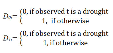
• Drought influences income and the food security of households. Years with below minimum rainfall, less than 300 mm/year were considered drought years and those above 300 mm/year were normal years. These swings necessitated the use of a shift dummy to take care of the dramatic changes in total income per adult equivalent, thus:
• Maize is a staple crop and contributes about 50% of daily caloric intake for most households in both counties. Thus, more maize production means higher household income [10].
• Ratio of area under maize to total cultivated area is likely to influence household income. The greater the ratio, the more likely greater maize production and consequently higher income.
• Livestock offtake refers to the percentage of the current year’s herd that is removed through sales, deaths, gifts, homeslaughter, or even theft. Higher offtake for the market or consumption would mean higher income and better food security.
• Beef price influences income. When prices are high, more is likely to be produced for sale, thereby increasing income.
• Higher maize prices are likely to stimulate maize production leading to increased income.
• Stocking rate refers to the number of livestock units grazed per unit area of land over time. Correct stocking rate ensures correct intensity of utilization of available forage and water. Animal numbers above optimum stocking rate would adversely affect the performance of other animals, causing a drop in output [11].
• Human population usually influences agricultural production and household income. Higher human population implies more labour availability; higher labour availability is likely to be engaged in more production of crops and livestock products, thus increasing income.
Model selection
Three models were tested to determine the one that fit the data best. These were the Ordinary Least Squares (OLS), Generalised Least Squares (GLS) and Autoregressive models. OLS is based on the assumption that the independent variables (X) and the dependent variable (Y) have a uni-directional relationship [12].
The OLS involves direct application of the base equation and all the classical assumptions on the error term are assumed to hold.
However, these assumptions can easily be violated in time series data. An AR model has its dependent variable lagged and used as an explanatory variable. For example, an output of a product today may affect its future output, and the current value of the output depends on the previous value [13]. The dependent variable follows a first-order autoregressive, or AR stochastic process, thus the value of the dependent variable at time t depends on its value in the previous time period and a random term, and is expressed as deviations from their mean value [14].
Lastly, the GLS model estimates the variances of the observations that are unequal (heteroscedasticity) or correlated by standardising the scale of the errors and “de-correlating” them. As opposed to OLS and AR, GLS detects the presence of autocorrelation, through Durbin Watson Statistics and Unit Root Test using the Cochrane-Orcutt procedure. The GLS is expressed as:
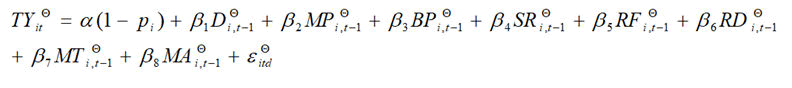
Where:
TYit=Total income per adult equivalent for each county at time t
Di,t-1=Drought lag 1residuals at time t
MPi,t-1=Maize price per kg lag 1residuals at time t
BPi,t-1= eef price per kg lag 1residuals at time t
SRi,t-1=Stocking rate lag 1residuals at time t
RFi,t-1=Rainfall amounts lag 1residuals at time t
RDi,t-1=Number of rain days in a year lag 1residuals at time t
MTi,t-1=Maize production in metric tonnes lag 1residuals at time t
MAi,t-1=Area under maize production lag 1residuals at time t
HLi,t-1=Labour lag 1residuals at time t
Ԑit=Error term at time t
θ=Differenced variables and error term
The Durbin-Watson statistic (d) detects the presence of autocorrelation, between values separated from each other by a given time lag in the residuals (prediction errors) from a regression [15]. However, for the AR model, the h-value, rather than the d-value, is used to test for the existence of autocorrelation due to the inclusion of a lagged depended variable as an explanatory variable [16].
A value of d=2 indicates no autocorrelation while d<2 is evidence of positive serial correlation and d>2, shows that successive error terms are negatively correlated [17]. On the other hand, if the h-value, tested at 5% level of significance, lies below -1.96, one cannot fail to reject the hypothesis that there exists negative serial correlation of the error terms; and if it lies above 1.96, the existence of positive serial correlation is suggested [18].
A unit root test was conducted to further test for stationarity (or non-stationarity) of the observations. The starting point is the unit root (stochastic) process illustrated as:
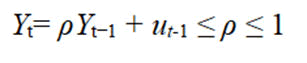
Where utis a white noise error term. If ρ=1, that is, in the case of the unit root, becomes a random walk model without drift, confirming a non-stationary stochastic process. Further, Dickey- Fuller (DF) test was carried out to find out if the estimated coefficient of Yt-1 is zero or not. The first level difference for each independent variable was regressed against its first order lag to obtain the t-value. This was then compared to the t-value generated with the DF table values. If the t-value is greater than the DF-value, then the data do not exhibit random walk [19].
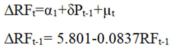
To illustrate with the rainfall amounts, the following equation was used:
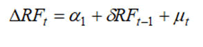
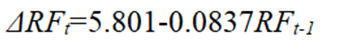
Where ΔRFt is the first-difference of the rainfall amounts, and the null hypothesis is set at Δ=0. If there was a unit root problem in the data, Δ would be equal to zero. The results were as follows:
The Kajiado County total annual rainfall (Pt):
t=(0.837) (-7.942)
r2=0.700; d=2.139
The Makueni County total annual rainfall (Pt):
t=(0.689) (-5.026)
r2=0.689; d=1.944
Since the error term is not autocorrelated based on the d-test the stationarity of deflated prices can be proved by the DF-test using the t-value. As can be seen from the estimated equation, at a significance level of 5%, the data did not exhibit random walk [20].
Descriptive analysis
The trends of the variables used in the time series analysis are presented. The data indicate that livestock offtake ranged between 14.1% in 1980 and 41.9% in 2009 for Kajiado and Makueni Counties respectively. The lowest livestock offtake reported in mid 1980s was linked to the droughts of 1983/84.
The situation is repeated immediately after 1991/1992 and 1995/96 periods, which were also periods of drought; and 1997/1998, which was a year of El Nino rain that resulted in flooding leading to loss of pasture and diseases such as pneumonia and foot rot, resulting in losses in livestock, and consequently reduced income [21].
Annual rainfall had links with livestock offtake per ha. From the early 1980's to early 1990's, these two exhibited a similar trend. However, from the mid-1990's to 2005, both depicted divergent trends, after which they continued to show a more similar trend. The explanation could be that in the 1980's to 1990's, rainfall patterns were more predictable and households in Kajiado County were able to adequately plan their pastoral way of life. From 1990 to 2004, rainfall became more erratic and unpredictable. With more rainfall, pasture and water were more available, leading to a reduction in livestock offtake. Among the pastoral households of Kajiado County, the Maasai tend to dispose of more of their animals to the market before they lose their body condition or die.
Total income showed no clear relationship with human population. In the early 1980's to 1990's, human population generally showed some growth, but at a very slow pace. Similarly, total income has continued to show a slow general growth, albeit with some gentle upward and downward swings (Figures 2 and 3).

Figure 2: Trends in offtake, annual rainfall, rain days, beef prices, maize prices, human population and income per adult equivalent in Kajiado Country, 1980-2010.

Figure 3: Trends in offtake, annual rainfall, beef prices, maize prices, human population and income in Makueni County from 1980 to 2010.
Beef prices have generally shown an increasing trend since the 1980's. The lowest beef prices were reported in 1984/1985, 1999/2000 and 2004/2005. These years coincide with the drought periods, as reported. The probable reason is that when rainfall is adequate, most pastoralists tend to hold on to their livestock. Conversely, many pastoralists sell off their livestock to minimise the devastating effects of drought. This makes beef prices to drop leading to reduced income.
Maize price has been highly variable. From the early 1980's to 1989, maize price was fairly stable but variability has increased since then. The highest maize prices were reported in 1985, 1987, 1992, 1997, 2005 and 2009. These periods correspond to just before drought or just after drought. For instance, the 1983/1984 drought affected agricultural production in 1985; thus maize prices shot up due to reduced maize production. The likely reasonis that climate parameters such as rainfall have a lagging effect and may not affect agricultural production in the same season.
Total income has continued to increase but with down-swings in 1984, 1994, 1997/1998, 2001 and 2007. These downswings in total income correspond to periods of weather extreme events such as droughts (1984, 1994 and 2001) and flooding (1997/1998). However, the decline in income noted in 2007 may have been caused by post-election violence that saw many people lose their property and assets.
Stocking rate has been declining irrespective of the rainfall levels. This implies that there are factors other than rainfall influencing stocking rate. Some of these factors may include size of land holdings, government policies and legislation. On the other hand, human population has shown an upward trend, though a decline was noted in 2004. This decline would not be verified, but one probable reason is that since population census is carried out every 10 years, the 2004 year was a poor estimate.
Real beef and maize prices have also shown some degree of trending with rainfall. When rainfall levels are low, maize and beef prices are high. This can be explained by the fact that during periods of low rainfall, drought limits moisture availability to crops, leading to reduced output and total income. For beef, at the onset of drought, prices will be low, since most households will be offering their livestock for sale. However, as the intensity of drought increases, fewer animals are offered for sale, reducing the supply of animals available for slaughter thereby pushing up the prices.
In addition, the plots of trend showed variability (zig-zag shapes) in annual rainfall, stocking rate, and real maize and beef prices. The trends in annual rainfall and maize prices support results from the USA, which showed that high variance in climatic conditions results in greater variability in crop yields and prices. Similarly, high livestock offtake were noted in periods of droughts (1983/84, 1987, 1992/93 and 2009), and floods (1997/98). This implies that during extreme weather events, households tend to dispose of their animals, and hold onto a few that could be sustained during the period. Also, in the early 1980's, livestock offtake continued to increase with real beef prices and maize prices irrespective of the rains, indicating that prices and other socio-economic factors rather than climate triggered this increase. Likewise, there have been downswings in livestock offtake, though the general trend has been upward. This shows that offtake trend closely follows real beef prices. It can be noticed that stocking rate is not influenced by rainfall levels and prices. Land being allocated to stock units is declining compared to the1980's. Further, the year 1994 had the lowest stocking rate, and the likely reason is that the 1991/1993 drought may have resulted in deaths of livestock, leading to lower stocking rates in the subsequent year. There was a marked increase in stocking and offtake rates between 1990 and 2010. In this period real beef prices rose steadily. The rise in real beef prices and the accompanying improvement in stocking and offtake rates occurred after the liberalisation of the beef markets in the late 1980's when producer and consumer prices were decontrolled, and at the beginning of the 1990's when a total waiver of controls in the beef and dairy industries in the country took place.
The contribution of different economic activities to the total income per adult equivalent is presented in Table 1. In Kajiado County, livestock was the greatest contributor (78.2%) to the total income per adult equivalent with remittances being the least; while for Makueni County, the greatest proportion was from crop production followed by livestock, and the least being remittances.
| Economic activity | Kajiado (Kshs) | Makueni (Kshs) |
|---|---|---|
| Farm-based | ||
| Livestock | 810 (78.2) | 581.0 (38.2) |
| Crops | 71.4 (6.9) | 802 (52.7) |
| Non-farm based | ||
| Employment | 117 (11.3) | 12 (8.2) |
| Remittances | 37.3 (3.6 ) | 14 (0.9) |
| Total | 1,035 (100.0) | 1,521 (100.0) |
Table 1: Contribution of different economic activities to total income per adult equivalent in Kajiado and Makueni counties.
The total income per adult equivalent was higher for Makueni County (Kshs 1,521), which is predominantly agropastoral, compared to Kajiado County (Kshs 1,034 per adult equivalent), a typical pastoral setting. Comparing these values to the recommended rural poverty line of Kshs 1,239 per adult equivalent, Makueni County households were likely to be less vulnerable to food insecurity than their counterparts in Kajiado County. This could be because Makueni County is a predominantly mixed farming area, growing both crops and livestock, which act as insurance for each other. For instance, when prices of cereals are expected to increase due to drought, farmers in Makueni County may hold on to their cereals and use it for consumption rather than for sale. Conversely, for Kajiado County, when there is drought, pastures become limited and livestock are often sold at through away prices. At this time, cereal prices shoot up. This reduces the purchasing power of households thereby increasing their vulnerability to food insecurity. The summary of the variables included in the regression analysis are presented in Table 2.
| Variable | Kajiado | Makueni | |||||
|---|---|---|---|---|---|---|---|
| Unit definition | Mean | Minimum | Maximum | Mean | Minimum | Maximum | |
| Dependent variable | |||||||
| Total income per adult equivalent | Kenya shillings | 1034 | 523 | 1477 | 1,521 | 785 | 2,216 |
| Explanatory variables | |||||||
| Total annual rainfall | Decimetre (dm) | 45.9 | 22 | 76.9 | 57 | 23 | 103 |
| Rain days | Days | 57 | 30 | 88 | 62 | 30 | 88 |
| Mean temperatures | Degrees celsius | 28.1 | 18 | 38 | 25 | 20 | 32 |
| Area under maize | Hectares | 28,987.8 | 9,300.0 | 44800 | 78,794 | 45,000.0 | 147,350.0 |
| Maize producer price | Kenya shillings/kg | 24.9 | 8 | 55 | 4.7 | 3 | 6 |
| Maize production | Metric tonnes | 43,219.7 | 1,946.0 | 64890 | 55778.6 | 11,251.0 | 96401.0 |
| Real beef prices | Kenya shillings/kg | 4.3 | 1.8 | 7.5 | 4.3 | 1.8 | 7.5 |
| Stocking rate | Tropical livestock unit | - | - | - | 4.7 | 2.9 | 6.5 |
| Labour | Human population | 326,399.3 | 40,500.0 | 59,8365 | 677,110.8 | 446.430.0 | 919,024 |
| Livestock offtake/ha | Tropical livestock unit | 6.2 | 3.2 | 12.7 | 5.6 | 2.4 | 9.6 |
| Livestock offtake | Per cent | 5.6 | 2.4 | 9.6 | 19 | 4.1 | 31 |
Table 2: Summary of variables used in the regression analysis.
Regression results
The climate factors represented in the models include mean annual rainfall, rain days and mean annual temperature. Table 2 reports the OLS, AR and GLS results for Kajiado and Makueni respectively, which represent the best outcomes, by considering the number of significant variables, adjusted (Adj) R2, F, and d values. In most of the regressions, the signs of the variables seem to be consistent. The OLS model is a poor fit for the data because of the high R2 for both Kajiado and Makueni Counties which cannot be explained by the very few significant explanatory variables. Further, the d statistics for the two data sets were less than 2; thus confirming the problem of positive serial autocorrelation. The AR model is an improvement on the OLS model because of the higher number of significant variables. However, the h value for the model lies outside the acceptable bounds of -1.96 and 1.96, suggesting the existence of (positive) serial correlation for both Kajiado and Makueni data sets. The model has also fewer significant variables compared to the GLS model. This then leaves us with the GLS model, which seems to represent the data best.
Table 3 reports the OLS, AR and GLS results for Kajiado and Makueni respectively, which represent the best outcomes, by considering the number of significant variables, adjusted (Adj) R2, F, and d values. In most of the regressions, the signs of the variables seem to be consistent. The OLS model is a poor fit for the data because of the high R2 for both Kajiado and Makueni Counties, which cannot be explained by the very few significant explanatory variables. Further, the d statistics for the two data sets were less than 2; thus confirming the problem of positive serial autocorrelation. The AR model is an improvement on the OLS model because of the higher number of significant variables. However, the h value for the model lies outside the acceptable bounds of -1.96 and 1.96, suggesting the existence of (positive) serial correlation for both Kajiado and Makueni data sets. The model has also fewer significant variables compared to the GLS model. This then leaves us with the GLS model, which seems to represent the data best.
| Variables | GLS model | AR model | OLS model | |||
|---|---|---|---|---|---|---|
| Kajiado | Makueni | Kajiado | Makueni | Kajiado | Makueni | |
| Constant | 0.33 | 0.88 | -1.42 | -2 | -2 | -2.96 |
| Human population | -0.93 | -0.8 | -0.96 | - | 1 | - |
| Drought (Yes or No) | 1.35 | -1.7 | -1.75* | -1 | -1 | -0.75 |
| Lagged total annual rainfall | 3.56** | -1.97** | 0.97 | -1 | 1 | -0.45 |
| Rain days/per year | 0.71 | 1.4 | 0 | 1.55 | ||
| Maize price per kg | 3.10** | 1.43 | 2.31** | 1.3 | 1.89* | 1.21 |
| Beef prices per kg | 0.83 | 2.20** | 1.01 | 1.99** | -1 | 2.55** |
| Mean annual temperature | -3.70** | - | -1.65 | -0 | -2.01** | -0.08 |
| Area under maize cultivation | - | - | - | 0.5 | 1 | 0.59 |
| Maize production (metric tonnes) | 1.73 | - | 1.82* | -1 | 1 | -0.68 |
| Per cent livestock offtake | 4.71** | 4.98** | 2.79** | - | 4.46** | - |
| Livestock offtake/ha | - | - | 4.59** | - | 5.50** | |
| Rainfall days per year | 1.82* | 1.90* | - | - | - | - |
| Stocking rate | - | 4.40** | - | 3.20** | - | 3.27** |
| Lagged income/AE | - | 0.97 | 0.6 | - | - | |
| Kajiado: AdjR2=0.801, F=8.516 (p ≤ 0.05), d=2.098; | Kajiado: AdjR2=0.935, F=27.545 (p ≤ 0.05), h=37.97 | Kajiado: AdjR2=0.955, F=40.184, d=1.524 (p ≤ 0.05); | ||||
| Makueni: AdjR2=0.813; F=10.886 (p ≤ 0.05), d=1.9991 | Makueni: AdjR2=0.970, F=53.48 (p ≤ 0.05), h=36.41 | Makueni: AdjR2=0.954, F=60.769, d=1.475 (p ≤ 0.05) | ||||
Note: **Significant at p ≤ 0.05, *Significant at p ≤ 0.10
Table 3: Results of regression models for Kajiado and Makueni Counties.
In Makueni County, lagged rainfall had a negative and significant (p ≤ 0.05) influence on total income. It implies that an increase in rainfall leads to a decrease in total income. The negative effect may occur if the rains are too high and cause floods, resulting in reduced crop production and pasture growth. Some parts of Makueni County are prone to flooding and this may explain the negative effects of the total rainfall. Alternatively, since total income is from various sources, including remittances, the flows from other sources might be reduced during times of high rains due to expectations of adequate harvests. In contrast, Tasokwa found a negative influence between rainfall and maize production in Malawi. She reported that a decrease in rainfall due to droughts results in a decrease in maize production, as expected. Also, Raddatz acknowledges the role of rainfall shocks on agricultural output. His work reveals the importance of weather shocks especially droughts, extreme temperatures and windstorms to the overall growth performance in low income countries like Nigeria. Further, established that in Ghana annual rainfall levels and their temporal distribution have a far-reaching impact not only on water availability and quality but also on crop yields, consequently influencing food security at household and national levels.
Other variables that were significant at p ≤ 0.05 in Kajiado County were maize price, temperature and livestock offtake. Maize price has a positive response to total income. It is understood that with higher maize prices, less food will be purchased with the available income. However, the households that grow maize along the river valleys or through irrigation normally have higher incomes due to higher maize producer prices. Similarly, for these households that grow maize, higher maize prices imply that more income would be available to purchase extra livestock, which would increase their capital base. The mean annual temperature exhibited a negative and significant (p ≤ 0.05) relationship with income per adult equivalent in Kajiado County. Since the county is mainly involved in livestock production, this implies that an increase in temperature will negatively affect the production of livestock, which will in turn lead to a decrease in total income. In support, showed that an increase in air temperature markedly reduced milk production levels in the central Great Plains of the United States unless counter-acting measures were taken by producers. He further elaborated that increased ambient temperatures led to depressed voluntary feed intake, thus reducing livestock output.
According to Osbahr and Viner, the annual average temperature in Kenya is projected to increase by between 3°C and 5°C by the end of the millennium because of climate variability and change. The increase in temperature brings consequences such as loss of moisture and increased evaporation rate. Coupled with declining precipitation, climate variability and change worsen the aridity of pastoral rangelands and affect a number of resources such as water, pasture and the edible fruits that pastoralists depend on. The ensuing consequences would be the decimation of livestock in large numbers, which could significantly affect pastoral livelihoods and security. This implies that the Kajiado County population is threatened with food insecurity if appropriate technologies and policies are not formulated.
The results of the current study are consistent with those of similar studies in other agricultural systems. For example, Tasokwa established that higher temperatures lower maize production. Also, Battisti and Naylor showed that an increase in temperature in the tropics may reduce maize and rice yields by 20 to 40 percent at the end of this century. Likewise, Schlenker and Roberts showed that in North-eastern US, an increase in temperature beyond a threshold of 30°C would result in sharp reduction of maize yields.
In lower altitudes, IPCC projects reduced crop productivity for even relatively small local temperature increases of 1°C to 2°C. In addition, IPCC projects that in the tropics and subtropics, crop yields may fall by 10°C to 20°C by the year 2050 due to warming and drying, but there are places where yield losses may be much more severe.
Stocking rate had a positive and significant influence (p ≤ 0.05) on total income in Makueni County. Nyariki noted that correct stocking rate ensures correct intensity of utilisation of available forage, water and other resources, and is therefore an indicator of capital investment and management quality. He further stated that if the stocking rates were too high, they would lead to overgrazing and possible range degradation. The positive effect of stocking rate on total income in the model indicates that there is a mismatch between livestock and the available forage. This implies that if stocking rates were to be increased, livestock production would increase and total income would also go up. In addition, Makueni County being an agricultural community, the crop residues at the end of every growing season complement natural pastures.
The results of this study have shown that total county income is influenced by climate variability (rainfall and temperature) in Kajiado and Makueni Counties of Kenya. Therefore, those involved in policy interventions should ensure that relevant climate data are collected and recorded for each specific area so that forecasting can be more accurate and can provide better guidance for designing appropriate adaptation strategies. Besides, climate factors are highly variable and thus strategies for adaptation cannot be generalised, and should therefore be more site-specific. Initiatives that promote the creation of microclimates such as agroforestry should therefore be encouraged and supported. This will help in moderating temperatures as well as attracting rainfall, while also offering other benefits, especially multipurpose trees and shrubs.
The regression analysis shows that per cent livestock offtake remains an important parameter for the livelihoods in both Kajiado and Makueni Counties. It had a positive and significant influence on total income for both counties. In Kajiado County, livestock contributed 78.2 percent of the county’s total income while in Makueni County it accounted for 38.2 percent. Therefore, development interventions geared towards livestock improvement have greater potential to improve total income. For example, decentralisation of bodies such as the Kenya meat commission, milk processing plants and leather industries to county level is fundamental. This will help minimise exploitation of farmers by middlemen. In addition, strengthening of extension services, provision of mobile veterinary care clinics, and improving education and awareness among the transhumant pastoralists and agropastoralists should be prioritised. Besides, relying on livestock sales alone may be unsustainable. There is therefore the need to create microindustries that deal with the processing of livestock related products (such as hides and skins to improve household income) as well as non-farm employment. Lastly, development initiatives that would specifically target Kajiado County should include implementing agroforestry and reforestation programmes to help moderate temperatures and attract more rainfall while also sequestering carbon.
Special thanks to Stockholm Environment Institute (SEI)-Africa Office for funding this study. Also special thanks to the various government departments, namely Kenya Meteorological Organisation, Ministry of Livestock and Fisheries, Ministry of Agriculture, and Kenya Institute of Policy and Research Analysis (KIPPRA), for availing data and information that were critical for this study. The teams of extension officers and field assistants in Kajiado and Makueni Counties are appreciated for their dedication in organising for data collection. Thanks also to the reviewers who shared detailed and useful comments.
The authors declare that they have no conflict of interests.
This article does not contain any studies with human or animal specimen performed by any of the authors.
[Crossref] [Googlescholar] [Indexed]
[Crossref] [Googlescholar] [Indexed]
[Crossref] [Googlescholar] [Indexed]
[Googlescholar] [Indexed]
[Googlescholar] [Indexed]
[Googlescholar] [Indexed]
[Googlescholar] [Indexed]
[Crossref] [Googlescholar] [Indexed]
[Crossref] [Googlescholar] [Indexed]
[Crossref] [Googlescholar] [Indexed]
Citation: Amwata D, Nyariki DM (2022) Causes of Household Vulnerability to Food Insecurity in Semi-Arid Kenya: Application of a Stationary Stochastic Model. J Agri Sci Food Res. 13: 505.
Received: 21-Jun-2021, Manuscript No. Manuscript No. JBFBP-21-10775; Editor assigned: 25-Jun-2021, Pre QC No. JBFBP-21-10775 (PQ); Reviewed: 09-Jul-2021, QC No. JBFBP-21-10775; Revised: 30-Nov-2022, Manuscript No. JBFBP-21-10775 (R); Published: 17-Mar-2023 , DOI: 10.35248/2593-9173.23.14.134
Copyright: © 2022 Amwata D, et al. This is an open-access article distributed under the terms of the Creative Commons Attribution License, which permits unrestricted use, distribution, and reproduction in any medium, provided the original author and source are credited.