Journal of Defense Management
Open Access
ISSN: 2167-0374
ISSN: 2167-0374
Review Article - (2021)Volume 11, Issue 5
This two-part guide reviews several standard data analytic tools with a wide variety of military financial management applications. Consider defence fuel budgets. The better our budget estimates, greater the efficiency and effectiveness of our forces. Budgeting too little can impact future operations, training, equipment, or sacrifice other priorities reprogrammed to fill funding gaps. Budgeting too much also risks sacrificing military priorities, as extra funds may be discovered too late to be reprogrammed efficiently. To minimize costly adjustments and wasteful reprogramming requires better guesses. The challenge with fuel prices is that they vary a lot. We have three choices, to: Ignore variability, Capture variability, or explain variability. The first section reviews extrapolative Forecasting and Sample Means (Averages) that mostly ignore variability, and then proceed to Confidence Intervals and Critical Values that attempt to capture variability. The next section explores the power of Simulation and Regression Analysis (“parametric estimation”) that tries to explain variability. This two-part guide briefly summarizes each approach in the context of fuel budgets, together with hints of how to apply the techniques in Excel. Widespread application of these and other data analytic tools could improve military management and budgeting and increase the efficiency and effectiveness of our forces.
Military financial management; Military services; Forecasting; Simulation and regression analysis; Budgeting
“It's tough to make predictions, especially about the future.” Yogi Berra
Yogi Berra was right. It’s tough to make predictions. An important application is defence budgeting. Uncertainty over costs and future funding is especially problematic for the military. Defence departments typically program resources (equipment, personnel, and funding) years in advance.13 A nation’s security critically depends on the accuracy of these forecasts.
The better our budget forecasts, the greater the potential efficiency and effectiveness of government programs. Forecasting fuel budgets offers an illustration. This two-part guide reviews several standard data analytic techniques with a wide variety of management applications. Each technique is briefly summarized in the context of budgeting for fuel, together with hints of how to apply the technique in Excel.
The fuel budget case study serves to review and summarize eight possible guesses, generated from six standard data analytic techniques. The techniques start simply. We launch the first of this two-part series with extrapolative Forecasting and Sample Means (Averages) that mostly ignore variability, and then proceed to Confidence Intervals and Critical Values that attempt to capture variability. The next section explores the power of Simulation and Regression (or “parametric estimation”) which attempt to explain variability.
Consider the risks of under- or over-Programming military funding for: Equipment (Procurement), Research & Development (R&D), Construction (MILCON), Military Personnel (MILPER), or Operating & Maintenance expenses (O&M). Fuel budget forecasts in the U.S. are included in the O&M account. The better our estimates, the more accurate our programming and budgeting, the greater the efficiency and effectiveness of future forces.
Regrettably, the U.S. Government Accountability Office (GAO) routinely criticizes the Department of Defense (DoD) for its cost and budget estimates. This two-part guide presents several data analytic approaches to improve those estimates. Widespread application of these and other analytical tools & techniques can improve military.
Reducing uncertainty to improve budget estimates involves three fundamental questions: 1) what can go wrong? 2) How bad is it? and 3) what are the chances? In answer to the first question, two things can go wrong. The dual risk is: i) Underestimating future expenditures and Programming too little; or ii) Overestimating future expenditures, and Programming too much. In the case of U.S. fuel budgets:
E]ach fiscal year, the Department of Defense (DOD) sets a standard price…it will charge the military services... In setting this standard price, DOD endeavors to closely approximate the actual price it will pay for the fuel during the year of budget execution. However, due to the timing of DOD’s budget process, the department estimates this price almost a year in advance of when it will actually purchase the fuel…
If the actual market price…is higher than the price DOD is charging its [military] customers, DOD will have to pay more for fuel than it is being reimbursed [i.e., DoD underestimates future expenditures]. If the actual price is lower than the standard price, DOD will have more cash than it anticipated [i.e. DoD overestimates future expenditures]. (GAO 2014 p.1) [1].
The second question “how bad is it?” explores the consequences:
i) Underestimating future expenditures and Programming too little can have serious consequences. For example, GAO (2015) reports early deliveries of the U.S. Air Force F-35 Joint Strike Fighter experienced nearly 50% cost overruns (from an original guess of $226,355mil to $338,950mil). Programming too little can impact future quantities, quality, or sacrifice other government priorities reprogrammed to fill funding gaps [2,3].
ii) Overestimating future expenditures and Programming too much can also have serious consequences. Surprisingly, GAO (2015) found the U.S. Navy’s DDG1000 Destroyer enjoyed a nearly 40% cost under run (from an original guess of $36,858 mil to $22,497mil). But programming too much can sacrifice other priorities, as extra funds may be discovered too late to be reprogrammed efficiently and effectively.
In the case of fuel, GAO (2014) cites a DoD study that warns: “Fuel cost volatility poses a major threat…and can require funding reallocations that disrupt investment programs or threaten readiness.” (p.35) to minimize costly adjustments and wasteful reprogramming requires better guesses. This leads to the third question—what is the likelihood? This data analytic guide offers eight ways to improve budget estimates and reduce the risk of under- or over-programming defence expenditures [4,5].
Section I: Ignore or capture variability
Consider fuel prices. With no uncertainty, it’s easy to make predictions. If prices never vary and the future mirrors the past, simply use the latest price paid to estimate next year’s fuel costs. But prices vary a lot, sometimes wildly. For instance, in 2012 DoD under-estimated actual fuel prices by nearly 30%: “DOD estimated a standard price of $131.04 per barrel [while] DOD’s actual costs averaged $167.33 per barre.” (GAO 2014 p.8) Two years later DoD vastly over-estimated fuel prices when oil prices collapsed to $60/ barrel, paying nearly $14 billion for the equivalent of 87 million barrels—an average cost in excess of $160/barrel:
During fiscal years 2009 through 2013, the DOD’s actual costs for bulk fuel differed considerably from its budget estimates, largely because of fluctuations in fuel prices...DOD underestimated its costs [fuel budgets] for 3 years [2010 -$2.9bil; 2011 -$3.4bil; 2012 -$3.2bil] and overestimated them for 2 years [2009 +$3.0bil; 2013 +$2.0bil] (GAO 2014 p. 1).
Fuel costs provide a convenient case study to illustrate several standard data analytic approaches to improve incremental public budgeting— with one important caveat. The data analytic techniques\ reviewed here represent “the tip of the iceberg.” Faced with the challenge of an actual fuel budget forecast, defence analysts apply some combination of these tools, together with other data analytic techniques [6,7].
Consider a budget that consists of a price per gallon (P) multiplied by a quantity of gallons (Q): “DOD and the Military Services estimate total funding needs for fuel in annual budget requests by using planned consumption [Q]…and a standard price [P]…set by DOD.” (GAO 2016). How much should we program for next year’s fuel costs? In fiscal year, t, and our prediction of next year’s (t+1) budget is: Bt+1=Pt+1 x Qt+1.
“GAO identified two factors that contributed to the differences between estimated and actual costs— (1) fuel price fluctuations [Prices (P)] and (2) differences between the military services’ estimated fuel requirements and their actual fuel consumption [Quantities (Q)]… [D]ifferences between estimated and actual fuel costs were accounted for primarily by fluctuations in the market price for fuel.” (GAO 2014 p. 7) [8,9].
Suppose we know next year’s requirement, say Qt+1=100,000 gallons, but are uncertain about next year’s price, Pt+1 =? ($/gallon). What should we use as our price estimate? How much should we program for next year’s fuel budget?
We have three choices: A) Ignore variability; B) Capture variability; or C) Explain variability. The fuel budget case study serves to review and summarize eight possible estimates, generated from six standard data analytic techniques. The techniques start simply. We launch the first of this two-part series with extrapolative Forecasting and Sample Means (Averages) that mostly ignore variability, and then proceed to Confidence Intervals and Critical Values that attempt to capture variability. In the next section we explore the power of Simulation and Regression or (“parametric estimation”) which attempt to explain variability. Each technique is briefly summarized, together with hints of how to apply the technique in Excel.
We will generate eight predictions of next year’s fuel budget (Bt+1) from our six data analytic techniques. But there is a catch. As we move from ignoring variability, to capturing variability, and finally explaining variability, we may enjoy progressively more confidence, but sacrifice precision. To increase both confidence and precision requires more data, better data, and/or more sophisticated data analytic techniques, which takes time and money.
A) Ignore variability
1. First guess=> extrapolative forecasts: With no data on past prices, we could use the latest spot market price, P as our estimate. In the simplest case, if this month’s price is P =$2.50/ gal, a first guess of next year’s budget is: Bt+1=$250,000.
2. If Pt+1 =  =$2.50/gal, and Qt+1=100,000 gallons: B1 = $250K
Second guess=> sample mean: Collecting data on past prices,
we could use the average (or “mean”) of our sample of
n=1, N prices as our estimate.14 Given N=36 months of
prices in Table 1, the Average Price is  15 (See Excel Hint) So, our second guess is:
Bt+1=$200,000.
| 2.50 | 2.04 | 1.11 | 2.10 | 1.95 | 2.02 |
| 2.56 | 2.81 | 2.54 | 1.91 | 0.58 | 1.61 |
| 1.60 | 2.48 | 2.25 | 2.33 | 1.86 | 2.90 |
| 2.90 | 2.82 | 1.45 | 2.62 | 1.07 | 1.84 |
| 1.51 | 1.38 | 1.97 | 2.06 | 2.15 | 0.97 |
| 2.25 | 2.08 | 2.59 | 1.66 | 1.31 | 2.05 |
Table 1: Sample of N=36 months of prices ($/gallon).
● If Pt+1 = P= $2.00/gal, and Qt+1=100K gallons: B2 = $200K (Table 1).
Note: An Average (or “Mean”) is calculated in Excel inserting data into the formula Average (number1, number2)
Excel hint: To calculate the average (or mean), first type the 36 months of prices found in Table 1 into a single column in Rows A1 through A36 (going down each column, starting with the most recent observation $2.50/gallon). Then click into cell A37 and type: =Average (A1:A36)
Table 2 re-organizes the data in Table 1 based on the frequency (count), and relative frequency (probability), of prices in our sample. Recall that to create Frequency and Relative Frequency data requires the selection of price intervals. Ten intervals are reported in Table 2. Next, we record the number of prices in Table 1 that appear in each interval. That is the count or “Frequency” recorded in the second column of Table 2. The “Relative Frequency” in the third column is simply the count (frequency) divided by the number of observations (N=36).
| Cost ($/gal) | Frequency (Count) | Relative Frequency (Count/N) |
|---|---|---|
| ≤1.2 ($1.20) | 4 | 11% |
| 1.2-1.4 ($1.40) | 2 | 6% |
| 1.4-1.6 ($1.60) | 2 | 6% |
| 1.6-1.8 ($1.80) | 3 | 8% |
| 1.8-2.0 ($2.00) | 5 | 14% |
| 2.0-2.2 ($2.20) | 7 | 19% |
| 2.2-2.4 ($2.40) | 3 | 8% |
| 2.4-2.6 ($2.60) | 5 | 14% |
| 2.6-2.8 ($2.80) | 1 | 3% |
| ≥2.8 ($3.00) | 4 | 11% |
| N=36 | =100% |
Table 2: Frequency and relative frequency of N=36 prices.
Figures 1 and 2 offer graphical illustrations of the frequency distribution (count), and relative frequency (probability) distribution, of our sample of N=36 past prices reported in Table 2 (Figures 1 and 2).
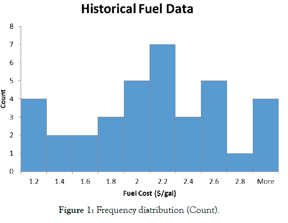
Figure 1: Frequency distribution (Count).
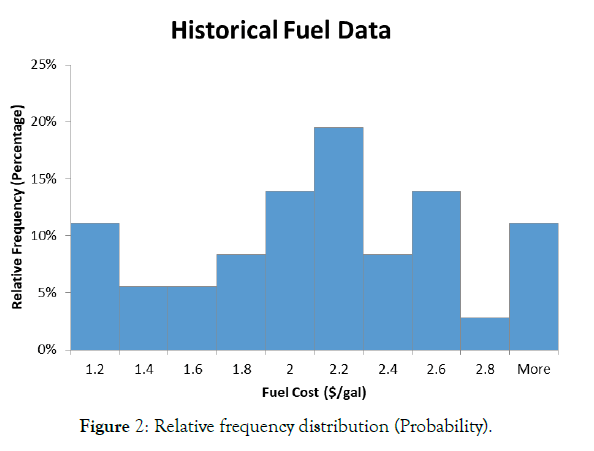
Figure 2: Relative frequency distribution (Probability).
Excel hint: To generate Frequency and Relative Frequency histograms (graphs) in Excel (Figures 1 and 2), first enter the ten intervals in parenthesis from the first column in Table 2 into Rows C1 through C10 of your Excel spreadsheet. Then click on the Data tab and choose the data analysis tool pack. Select Data Analysis, then Histogram. Next, click into the rectangle next to Input Range and type A1:A36 (alternatively, hit the square next to the rectangle, and block our column of N=36 fuel prices). In the Bin Range enter C1:C10 (or block our ten intervals). Next, check the Chart Output box and click OK. You should get a frequency graph similar to Figure 1. For Figure 2, select/highlight both the fuel cost interval and frequency columns. Click on the Insert tab and select the bar chart. You should get a relative frequency graph similar to Figure 2.
Note in Figures 1 and 2, how spread out our sample of N=36 past prices are around the average (mean) price P=$2.00/gal. Since past prices varied significantly around the mean, how confident can we be using the sample average to predict next year’s price (or fuel budget)? Instead of ignoring this variability, a better guess would attempt to capture variability. But this requires a measure of dispersion of data around the mean of the “population” from which our sample is drawn called the standard deviation (σ=sigma).
Note: A Standard Deviation (σ) is calculated in Excel inserting data into the formula STDEV (number1, number2)
Excel Hint: To obtain the standard deviation of our sample data (s), return to our 36 months of prices in the single column—Rows A1 through A36. Then click into cell A38 and type:=STDEV(A1:A36)
B) Capture variability
Two standard approaches to capture variability are through: Confidence Intervals and Critical Values. When to use one or the other? That depends on a useful distinction between “uncertainty” and “risk.”
• Uncertainty is the lack of perfect information about future measures of interest (e.g. fuel prices) and can be described using Confidence Intervals.
• Risk is the likelihood of undesirable outcomes (for example, exposure to budget shortfalls from underestimating future fuel expenditures and Programming too little) and can be described using Critical Values.
2. Third guess=> confidence intervals (C.I): Given uncertainty about next year’s fuel price, instead of using the sample mean (a point estimate) and hoping we get lucky, intervals can be constructed around the sample mean that offer some confidence the true (population) mean lies somewhere in those intervals.
Past price variability is captured in confidence intervals constructed
using a measure of dispersion of data around the population mean
called the population standard deviation (σ=sigma). The problem
remains that to build a confidence interval, we need something we
generally don’t know, the population standard deviation, and σ.
The best we have is our sample standard deviation, s. So, instead
of using σ to build confidence intervals, we adjust the sample standard
deviation (s), dividing it by the square root of the sample size
(n), and use what we call the “standard error”: 
Reports descriptive statistics for our sample of fuel prices (see Excel
Hint). Rounding up, the Mean of the sample is P=$2.00/gal, and
Standard Deviation is s=$0.60/gal. So, the standard error is:  = $0.60/6 = $0.10 (Table 3).
| Mean | 1.995 |
| Standard Error (S.E.) | 0.096 |
| Standard Deviation (s) | 0.577 |
| Sample Variance | 0.333 |
| Range | 2.311 |
| Minimum | 0.584 |
| Maximum | 2.895 |
| Count | 36 |
| Confidence Level (95.0%) | 0.195 |
Table 3: Descriptive statistics from sample of prices.
Excel hint: An easier way to obtain descriptive statistics for our sample (including the mean, standard deviation, etc.) is to use the Data Analysis Tool Pak. In our Excel spreadsheet simply click the Data tab, select Data Analysis, then Descriptive Statistics. Check Summary Statistics and then click into the rectangle next to Input Range and type A1:A36 (Alternatively, hit the funny box to the right, and block our column of fuel prices and hit Enter). When you hit OK, a column of summary statistics should appear similar to Table 3.
To build confidence intervals requires adding and subtracting standard errors (S.E.) from the mean. The more standard errors we add and subtract, the bigger the interval, and the greater our confidence (probability) the true population mean lies somewhere in that interval. In general, with large enough samples (n≥30), we can express:
68.26% confidence for an interval ± 1 S.E. around the sample mean, 95.44% confidence for an interval ± 2 S.E. around the sample mean, 99.74% confidence for an interval ± 3 S.E. around the sample mean.
This reveals a trade-off between confidence and precision. The greater confidence required, the bigger the interval (i.e. the less precision). To increase both confidence and precision requires more and/or better data, which takes time and money.
A popular confidence level is 95%. This corresponds to an interval
nearly two (±1.96) standard errors (S.E.= s/ n. = $0.10) around a sample mean (P=$2.00/gal). In general, the choice of confidence
level (partly) depends on the consequences of being wrong. Presumably,
the greater the consequences, the more confidence required.
Sadly, the greater confidence required, the bigger the interval, and
thus the “sloppier” our estimate. To obtain more precise estimates
(i.e shrinking the confidence interval) for the same confidence
level, requires more and/or better data. Otherwise, more precise
estimates can be obtained by accepting less confidence i.e. a greater
risk the true (population) mean lies outside our confidence interval.
To capture variability, with a sample mean P=$2.00/gal, and standard error S.E.=$0.10, the 95% Confidence Interval is [$2.00-(1.96 × $0.10); $2.00+(1.96 × $0.10)] = [$1.80; $2.20]. If our sample were truly random, then we can be 95% confident the true population mean of past prices lies somewhere between $1.80/gal and $2.20/ gal. Of course there is still a 5% risk the true mean value (average price) lies outside this interval. Therefore, based on our sample price data, if the future mirrors the past, we can be 95% confident the true population mean of next year’s fuel costs will lie somewhere in the interval: Bt+1=[$1.80 × 100,000; $2.20 × 100,000] =[$180,000; $220,000].
● If P=$2.00/gal, S.E.=$0.10, Qt+1=100K gallons, then the 95% C.I. is B3=[$180K; $220K]
Note: Excel calculates the value that needs to be added and subtracted from the mean to obtain Hi & Lo bounds of a Confidence Interval with the formula =CONFIDENCE (Alpha, Standard_dev, Size) [Alpha=1-Confidence Level; Standard_dev= Standard Error; Size= Sample Size]
Excel hint: Another way to obtain a Confidence Interval (C.I.) using our Excel spreadsheet is to click the Data tab, then Data Analysis, and select Descriptive Statistics. Check the box for Confidence Level for Mean and input whatever confidence level we need (for example, 95). Then click into the Input Range and type A1:A36. Hitting OK yields the value (for example, 0.20) we add and subtract from the mean to obtain the Hi and Lo bounds of our Confidence Interval.
A 95% Confidence Interval (C.I.) around our sample mean price appears below, along with three other confidence intervals:
50% C.I.= $2.00 $0.07=[$1.93, $2.07]=>$0.14/gal interval between
Hi & Lo
90% C.I.= $2.00
  $0.16=[$1.84, $2.16]=>$0.32/gal interval between
Hi & Lo
95% C.I.= $2.00 $0.20=[$1.80, $2.20]=>$0.40/gal interval between
Hi & Lo
99% C.I.= $2.00
 $0.26=[$1.74, $2.26]=>$0.52/gal interval between
Hi & Lo
These four Confidence Intervals illustrate the trade-off between confidence and precision. The greater confidence required, the less precision (i.e. the bigger the interval). For example, if we are willing to accept a 50-50 chance of capturing the true (population) mean price, then there is only a 14 cent/gal gap between the Hi and Lo bounds of the interval. Note the gap increases to 52 cents/gal if we need to be 99% confident the true mean price lies somewhere in the interval.
The dilemma is that budget estimates that attempt to capture variability using a C.I. necessarily involve interval estimates. For example, our sample price data suggests we can be 95% confident next year’s fuel expenditures will be somewhere between $180K and $220K (a $40,000 gap that reflects uncertainty). While this is useful information, for purposes of public budgeting, a single value must generally be selected. Unfortunately, if we select any value in the interval (say the mid-point $200K) we can no longer express any statistical confidence in that estimate.16 One way out of this dilemma is to shift from uncertainty to risk, and to use “critical values.”
4. Fourth guess=> critical values: Reporting an interval and expressing 95% confidence the budget we need next year lies somewhere in that interval can be problematic. Public budgeting typically requires point estimates, not interval estimates. While useful in calculating upper and lower bounds of possible programming errors,17 it can be helpful to reframe the problem to obtain a single price (or budget) estimate. The question then becomes: For any price estimate (or “critical value”) used to program next year’s budget, what is the Risk we will underestimate actual expenditures and program too little, and experience a budget shortfall? Or, for example, how much should we program for next year’s fuel costs to be 95% confident we will have sufficient funds, and only a 5% risk we will run over and need more?
The challenge is to identify a fuel price to use in our budget estimate, so there is only a 5% risk the actual price will be higher than this critical value. Programming next year’s fuel budget using this price would give us 95% confidence actual expenditures will lie at or below our requested budget, and only a 5% risk of a cost overrun (or budget shortfall).
For example, using our best guess of the population mean as our critical value (i.e. our sample average fuel price, P=$2.00), gives us 50% confidence the future price will be at or below this value, but also a 50% risk actual prices will be above this critical value. Figure 3 illustrates the risk of under-programming expenditures if we ignore variability and use the population mean price P=$2.00/ gallon, and program $200K for fuel. This budget estimate gives us 50% confidence we will meet actual expenditures next year, but also a 50% risk of a budget shortfall, or that actual fuel costs will exceed $200K (Figure 3).
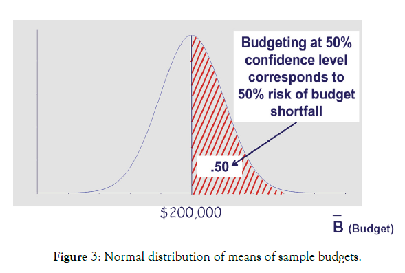
Figure 3: Normal distribution of means of sample budgets.
For any price estimate (critical value) we use to program next year’s fuel budget to achieve more than 50% confidence, our sample data allows us to determine the probability we will have sufficient funds, and the risk we won’t. But first it is necessary to convert our price estimate into a “Z-score.” Recall this measures how many standard errors our estimate is above the mean: Z-score = [(Critical Value–Mean)/Standard Error].
Note: Formula to find a Z-score (number of standard errors above the mean) in Excel is =NORM.INV(Probability, Mean, Standard_ dev)
For example, a fuel price estimate (critical value) of $2.00/gallon corresponds to a Z-score of 0, since it is zero standard errors above the mean. Since our standard error is $0.10, using $2.10 as our price estimate is one standard error above the mean, and corresponds to a Z-score of 1. Using $2.20, our guess is two standard errors above the mean, with a Z-score of 2. In fact, converting any price estimate into a Z-score allows us to calculate the probability we will have sufficient funds (called the “p-value”), and the risk we won’t (one minus the p-value).
Note: For any given price estimate (critical value), Excel calculates the probability (“p-value”) we will have sufficient funds using the formula =NORM.S.DIST(Z-score, True)
[Risk of facing budget shortfall is one minus this value] The example below illustrates declining risks of a budget shortfall (i.e. declining risks of under-programming fuel costs) for each of the corresponding fuel price estimates (Pt+1), and associated Z-scores:
50% Risk (50% Confidence): Pt+1=$2.00 (Z=0)
20% Risk (80% Confidence): Pt+1=$2.0845 (Z=0.845)
10% Risk (90% Confidence): Pt+1=$2.1285 (Z=1.285)
5% Risk (95% Confidence): Pt+1=$2.1645 (Z=1.645)
1% Risk (99% Confidence): Pt+1=$2.233 (Z=2.33)
1% Risk (99% Confidence): Pt+1=$2.233 (Z=2.33) Using a fuel price estimate of $2.00/gallon gives us a 50% risk of a budget shortfall. Suppose we need to lower the risk from 50% to 5%. How much should we program to be 95% confident there will be sufficient funds? What is the critical value?
Using the mean price P=$2.00/gallon (or Budget of $200K) gives us 50% confidence (or 50% probability) we will cover actual expenditures. The question is: How far above the mean (measured in standard errors: S.E.=$0.10) do we need to go to obtain an additional 45% confidence (probability) we can cover actual fuel expenditures (a total probability of 50%+45%=95%)? Using Excel (or a standard normal table), the critical value needs to be 1.645 standard errors (S.E.) above the mean. In this case, to be 95% confident we have programmed sufficient funds, the critical fuel price needs to be: $2.00 + (1.645 × $0.10) = $2.17.
Note: To obtain a Critical Value (Price Estimate) in Excel that corresponds with a designated confidence level (probability) of having sufficient funds, use the formula =NORM.INV (Probability, Mean, Standard_dev) [For 5% Risk: Probability=95, Mean=2.00, and Standard_dev=0.10]
Our fourth guess illustrated in Figure 4 indicates we can have 95% confidence in programming a fuel budget of Bt+1=$2.17 × 100,000=$217,000 with only a 5% risk of a budget shortfall.
● If P=$2.00/gal, S.E.=$0.10, Qt+1=100K gallons, the critical value for 5% under-programming Risk (or 95% Confidence of sufficient funds) is B4=$217K. (Figure 4).
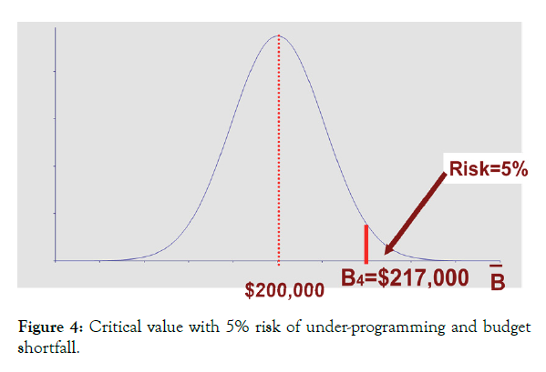
Figure 4: Critical value with 5% risk of under-programming and budget shortfall.
Interestingly, the U.S. weapon systems acquisition reform act (WASARA) requires:
Disclosure of confidence levels for baseline estimates of major defense acquisition programs.—
The Director of Cost Assessment and Program Evaluation, and the Secretary of the military department…shall each— (1) disclose … the confidence level used in establishing a cost estimate for a major… program, the rationale for selecting such confidence level, and…the justification for selecting a confidence level of less than 80 percent [or greater than 20 percent risk of under-programming.]
WSARA Public Law 111-23—May 22, 2009
Unfortunately, lowering the risk of a budget shortfall by selecting a confidence level greater than 80% creates another risk. For example, whereas our 95% confidence level satisfies WASARA mandates, and lowers the risk of under-programming, it increases risks of over-programming!
Selecting a confidence level greater than 80% lowers the risk of budget shortfalls (e.g. 95% Confidence=>5% Risk vs. 80% Confidence=> 20% Risk), but raises other risks related to over-programming: competing programs cannot be funded (within defense or other parts of government); inefficient end-of-year reprogramming; and/or higher costs if bigger budgets lower incentives to control costs. So, setting confidence levels not only requires evaluating acceptable risks of under-programming, but must also consider consequences of over-programming!
Section II: A data analytic guide for defence management and budgeting
Now what if we are uncertain about both the price and the requirement? For example, over the period 2009-2013 GAO (2014) found:
“[The] difference between the price DOD paid for fuel and the price it charged its [military] fuel customers…accounted for, on average, 74 percent of the difference between estimated and actual costs [fuel budgets]…[while] differences between the services’ estimated fuel requirements and actual fuel consumption…accounted for an average of 26 percent of the difference...” (p.8)
How much should we program for next year’s fuel costs when both variables (Price and Quantity) are uncertain?
1. Fifth Guess=> Simulation Model: Suppose we are not only uncertain about next year’s Price (Pt+1=? $/gal), but also the requirement Qt+1=? gallons). How much should we program for next year’s fuel budget: Bt+1= Pt+1x Qt+1=? Simulation offers a powerful tool when more than one variable is uncertain.
Simulation packages allow us to assign probability distributions to each variable (Price and Quantity), and to specify relationships between variables. (See Excel Hint and Appendices 1-3) Table 4 offers examples of some probability distributions that can be assigned to variables of interest. In our fuel budget case study, “Monte Carlo” simulations replicates real life with thousands of trials that repeatedly draw values from assigned probability distributions for price and quantity, and plot the resulting fuel budgets (B=P × Q). This generates a relative frequency histogram similar to Figure 2, which can be interpreted as a probability distribution of possible future fuel costs (Table 4).
| Beta | Student’s t |
| Chi-square | Exponential |
| Poisson | Triangular |
| Normal | Weibull |
| Uniform | Gamma |
| Lognormal | Logistic |
Table 4: Alternative probability distributions.
Our fuel budget case study assumes Prices are normally distributed and draws Quantities from a Triangular distribution (See Appendices 1-3). The relative frequency histogram (probability distribution) generated from the resulting budget (Price × Quantity) estimates can be used directly to capture uncertainty through confidence intervals, or to assess risk through critical values. For example, Figure 5 offers a notional relative frequency histogram (budget probability distribution) from a simulation of thousands of trials. To capture variability, we can either build a Confidence Interval that generates a fifth guess (B5a = [BLo; BHi]), or Identify a Critical Budget (B5b = BCritical) that offers an acceptable risk of a budget shortfall (Figure 5).
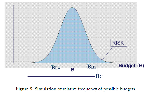
Figure 5: Simulation of relative frequency of possible budgets.
Excel hint: Building a Simulation requires commercially available Packages such as @RISK used with Excel. Appendix 1 describes how to identify and test which distribution to use as a model to best fit sample data such as our fuel prices. In @RISK, highlighting our Fuel Data column, select “Distribution Fitting” to fit a Normal Distribution. Appendix 2 describes how to generate a probability distribution model when we only have three data points (a Minimum, Maximum and Most Likely fuel requirement). Select “Distribution Fitting” to fit a Triangular Distribution. Finally, Appendix 3 describes how to define the relationship between our variables (Price × Quantity) in an Output Cell, and to run the simulation to generate results similar to Figure 5. To find upper and lower bounds of a confidence interval, or a critical value, simply slide the markers above the resulting budget relative frequency histogram (probability distribution) to generate charts similar to Figures 5a and 5b.
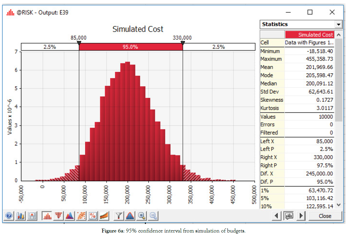
Figure 5a: 95% confidence interval from simulation of budgets.
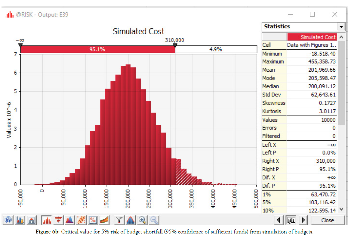
Figure 5b: Critical value for 5% risk of budget shortfall (95% confidence of sufficient funds) from simulation of budgets.
In the case of fuel prices (P), given our sample data, simulation packages allow us to test which probability distribution (e.g. Table 1) best fits the data. It turns out our sample fuel data fits a Normal distribution. (See Appendix 1) So, to simulate prices, we use a Normal distribution with the mean and standard error of our sample data (Mean=$2.00; S.E.= 0.10).
In the case of fuel consumption requirements (quantity in gallons, Q), suppose we have no data. In the absence of data, experts may be surveyed to reveal lower and upper bounds, and a most likely value. In our example, we assume the Most Likely requirement is 100K gallons. Suppose experts reveal the Minimum likely requirement is 75K gallons, and the Maximum 127K gallons. This is all we need to model next year’s requirement as a Triangular (or Beta) distribution. (Appendix 2)
Simulation software can be used to run thousands of trials which, in the case of fuel costs, repeatedly draws prices (P) from our normal distribution, and requirements (Q) from our Triangular distribution, and simply multiplies P × Q to generate and plot possible budgets. Figures 5a and 5b illustrate a relative frequency histogram (probability distribution) of possible budgets from a simulation of 10,000 trials. (See Appendix 3)
Confidence Interval: When both fuel prices and requirements are uncertain, results of the simulation illustrated in Figure 1a indicate we can be 95% confident next year’s expenditures will lie somewhere in the interval: Bt+1= [$85,000; $330,000].
● Given 36 months of fuel price data, and expert opinions on quantities (minimum likely requirement 75K gallons, maximum 127K, and most likely 100K), simulation results illustrated in Figure 5a reveal the 95% Confidence Interval: B5a=[$85K; $330K] (Figure 5a).
Note the gap between our Hi and Lo budget estimates ($330K- $85K=$245,000) reflects deep uncertainty about fuel costs. Given our sample data, the only way to shrink this gap is to accept less than 95% confidence the true budget (actual fuel costs) will lie somewhere in our interval. This reflects the unfortunate trade-off between confidence and precision. The more precision (smaller interval), the less confidence.
Instead of using a confidence interval (Lo and Hi budget numbers) to bound our guesses, it may be useful to shift our perspective from uncertainty to risk. This allows us to report a single “critical” value.
For example, the question may be how much to program for fuel (what is the “critical value”) so there is only 5% risk of a budget shortfall (or 95% confidence we will have sufficient funds)?
Critical value: When both fuel prices and quantities are uncertain, results of our simulation illustrated in Figure 5b indicate we can have 95% confidence there will be sufficient funds (or 5% risk of a shortfall) if we program a fuel budget: Bt+1=$310,000.
● Given 36 months of price data and expert opinions on quantities (i.e. minimum likely requirement of 75K gallons, maximum 127K gallons, and most likely 100K gallons), simulation results illustrated in Figure 1b indicate the Critical Value for 5% risk of a budget shortfall (95% confidence of having sufficient funds) is: B5b=$310K (Figure 5b).
Note that to accommodate the DoD mandate discussed earlier (WASARA 2009) of at least 80% confidence of having sufficient funds (i.e. no more than 20% risk of a budget shortfall), requires a budget of at least $255,000. According to our simulation, to increase confidence above 80% of having sufficient funds (or lower the risks of a budget shortfall below 20%), requires programming more than $255K for fuel.
Now suppose we know next year’s requirement, Qt+1=100,000 gallons, but are still uncertain about next year’s price, Pt+1=? ($/gallon). How much should we program for fuel: Bt+1= Pt+1 x Qt+1? The first two choices we explored include: A) Ignore variability; and B) Capture variability. The third and most data intensive choice is to: C) Explain variability.
C) Explain variability
Returning to the assumption we know next year’s requirement (Qt+1=100,000 gallons), instead of attempting to capture variability in our sample prices, what if we could explain the variability? Regression analysis, also known as “parametric estimation,” involves building a prediction model that includes factors (e.g. “cost drivers”) that help explain past variation in something we care about, i.e. next year’s fuel price.
6. Sixth guess=> regression analysis (Parametric estimation)
The goal is to construct a prediction model that helps explain past variation in fuel prices. The challenge is to uncover factors (explanatory variables) that account for this variation. The logic is simple. If these factors (e.g. “cost drivers”) adequately explain past variation, the same relationship might help predict the future. The regression relationship is your prediction model. Like any good relationship, building a regression takes some effort.
The U.S. Department of Energy’s “Energy Information Agency” (EIA) provides regular forecasts based on assumptions about factors related to energy prices. (www.energy.gov) Consider the following factors (explanatory variables) that might help explain variation observed in fuel prices:
● P=f (Supply, Demand, Wars, Weather, Exchange Rates, Cartels.)
For purposes of illustration, suppose energy supply is relatively stable, so that demand is the primary factor impacting prices (and assume other variables have negligible influence). With supply stable, world energy demand is likely one factor that influences prices. Demand for energy partly depends on the strength of the global economy. One “demand” measure (a so-called “proxy variable”) to help explain price volatility might be average economic growth rates of the world’s biggest economies—data routinely reported by the Organization for Economic Cooperation and Development (OECD).
Once we settle on one or more (“Independent”) explanatory variables, the next step is to consider the impact each explanatory variable has on our prediction (“Dependent”) variable, i.e. fuel prices. Is there a direct (positive) relationship between the two, or inverse (negative) relationship? Plotting the data, theoretical models, experience, judgment, and instinct are all valid guides. In our case, the hypothesis is that there is a positive relationship between economic growth rates and fuel prices: i.e. greater (smaller) growth rates correspond to increased (decreased) energy demand, reflected in higher (lower) prices.
Regression analysis offers a way to test the hypothesis that economic growth rates help explain variation in fuel prices. Applied regression analysis generally assumes a linear relationship exists at any time, t, between our dependent variable, fuel prices (Pt), and our independent (explanatory) variable, economic growth rates (Xt), or:
● Regression model: (Pt), = a + b (Xt), + (£t),
(Where “a” is the intercept and “b” is the slope of our linear
relationship, and  represents random errors from omitted
variables, etc.).
If there is a positive relationship between the Price (Pt), and Economic Growth Rates (Xt), then the slope coefficient “b” should be positive.
Given our sample of N=36 past prices Table 1, the challenge remains that to test our model requires the collection of corresponding data on economic growth rates over the same period. Table 2 offers an illustration (Table 5).
| 0.19 | 0.14 | 0.12 | 0.14 | 0.14 | 0.19 |
| 0.18 | 0.20 | 0.19 | 0.14 | 0.11 | 0.13 |
| 0.16 | 0.18 | 0.16 | 0.18 | 0.16 | 0.21 |
| 0.20 | 0.20 | 0.13 | 0.19 | 0.11 | 0.15 |
| 0.14 | 0.12 | 0.14 | 0.14 | 0.19 | 0.12 |
| 0.17 | 0.15 | 0.19 | 0.13 | 0.12 | 0.14 |
Table 5: Sample of N=36 months of global economic growth rates (%).
The next step is to enter data into a regression software package. (See Excel Hint and Table 6) Regression packages automatically report intercept (“a”) and slope coefficients (“b”) that generate the best linear relationship between the explanatory variable(s) and the prediction variable (i.e., the best linear relationship that minimizes the sum squared errors of actual fuel price data from what the model would predict).18 This best linear relationship is our prediction model. The logic is simple. If these factors adequately explain past variation, the same relationship might help predict the future.
| Regression Statistics | |||||
| R Square | 0.84 | ||||
| Standard Error (SEE) | 0.24 | ||||
| Observations (N) | 36 | ||||
| Coefficients | Standard Error | t Stat | |||
| Intercept (“a”) | -0.735 | 0.211 | -3.475 | ||
| X Variable (“b”) | 17.440 | 1.327 | 13.143 | ||
Table 6: Regression results.
Excel hint: To run our regression in Excel, first type the 36 monthly percentage global economic growth rates found in Table 3 into a single column in Rows B1 through B36 (going down each column, starting with the most recent observation, 0.19). Then click on the Data tab and find Data Analysis (as you did earlier to generate Descriptive Statistics). Scroll down the list to find Regression and click OK. Find Input Y Range (which is asking for our prediction variable—fuel prices), and insert A1:A36 into the rectangular space to the right and click Enter. (Alternatively, click the box next to the rectangular space and then highlight column A1 through A36 and click Enter…This automatically populates the rectangle with your fuel price data, A1:A36). Next find Input × Range (which is asking for our explanatory variable—growth rates), and insert B1:B36 into the rectangular space to the right and click Enter. (Alternatively, click the box next to the rectangular space and then highlight column B1 through B36 and click Enter…This automatically populates the rectangle with your growth rate data, B1:B36). Entering data was the hard part. Now all you have to do is hit OK. Regression statistics similar to those in Table 3 will automatically appear in a new sheet.
Regression results are typically reported in a table. Digesting the summary output takes a little practice. Table 6 reports regression statistics based on our sample of fuel prices and corresponding growth rates. Note Table 6 offers a streamlined version of regression results reported in Excel (Table 6).
Buried somewhere in the regression results are a set of coefficients (intercept and slopes). These are the keys to unlock our prediction model. These coefficients reveal the best linear relationship that exists between our explanatory variable (economic growth rates— X) and our prediction variable (fuel prices—P). The regression output reported in Table 6 reveals the best linear unbiased estimating (BLUE) relationship is given by:
(Pt), = a + b (Xt), = -0.74 + 17.44 (Xt),
A first guess: To obtain our first fuel price estimate, we must enter anticipated future values of our explanatory variables into our prediction model. So, before we can predict anything, we need educated guesses about future values of our explanatory variables. Any techniques previously discussed in this tutorial can be used to obtain these values. So to apply our regression model to forecast next year’s fuel price Pt+1 requires a prediction of next year’s economic growth rate Xt+1. Then simply enter the appropriate values into the prediction (regression) model and do the required multiplication and addition (Table 7).
| 0.18 | 0.17 |
| 0.18 | 0.19 |
| 0.17 | 0.17 |
| 0.17 | 0.15 |
| 0.15 | 0.13 |
| 0.17 | 0.15 |
Table 7: N=12 months of estimated future global economic growth rates (%).
From Table 7, the average of next year’s forecasted monthly growth rates is Xt+1= 0.17 which from our regression yields an estimated average annual price to use in next year’s budget estimate:
Pt+1 = -0.74 + 17.44 Xt+1 = -0.74 + 17.44 × 0.17 = $2.15,
Which generates a fuel budget (“point”) estimate:
● If Xt+1= 0.17, Pt+1= (-0.74 + 17.44 Xt+1)=$2.15, and Qt+1=100,000, then Bt+1= Pt+1x Qt+1= B6a=$215,000.
Before we place too much faith in this estimate, we need to ask a few questions:
• Does the data support our hypothesis of a direct (positive), or inverse (negative) relationship between a specific explanatory factor and the prediction variable? If not, why not?
• Since the (slope) coefficient on our explanatory variable (Xt) is positive
• (b=+17.44), this supports our hypothesis of a direct relationship between economic growth rates and fuel prices.
• Are the explanatory variables significant?
• If a slope coefficient is zero, the associated explanatory variable is useless (or redundant) in explaining past variation in fuel prices—it is not statistically significant. Although coefficients reported in regression outputs are never zero, that doesn't mean they're significant. Since reported coefficients are derived using sample data, reported coefficients are estimates, not true values, and have associated standard errors. The “t-statistic” reveals how many standard errors our coefficient value is away from zero. As a rule of thumb, a value two standard errors away from zero gives us roughly 95% confidence the coefficient is statistically significant (i.e. not zero). In Table 6, our intercept and coefficient values are more than 2 standard errors away from zero (i.e. the intercept more than 3 S.E. below zero, and slope more than 13 S.E. above zero). So far away in fact, that we can have more than 95% confidence in using those values to generate our forecast.
• How well does the prediction model explain the past variation observed in our prediction (dependent) variable?
• The best we could hope for is that our model explains 100% of past variation in fuel prices. The R squared statistic reported in Table 4 reveals the fraction of past variation explained by our model is 0.84. This means 84% of past variation in our sample fuel prices is explained by economic growth rates. An R squared measure lies somewhere between zero (the model is no help), and one (the model explains all past variation). The closer R squared is to one, the more confidence we can have in the model. But, be careful. It's possible to make useful predictions from models with low R squared, and useless predictions from models with high R squared. Let common sense prevail.
We now have a prediction model, and some appreciation of how good it is. However, we know from the R squared value that only 84% of past variation in fuel prices is explained by growth rates. (See Table 6) So some of the variation (16%) in our sample of fuel price data (the prediction variable) is not accounted for by the model i.e. depends on other explanatory factors. As a consequence much like using the average as our guess, point predictions from regressions are deceptively precise, or "exactly wrong."
A second guess: Building an interval much like a Confidence Interval, around our point prediction generates another guess that is "approximately right. This “prediction interval” accounts for both the point prediction and the unexplained variation (or error). Much like a confidence interval, prediction intervals are sloppier to report, since they involve a range of values. However, unlike our first forecast, we can express statistical confidence in this second forecast. The standard error of the estimate (SEE=$0.24) found in our regression results (Table 6) measures the unexplained variation. To obtain approximately 95% confidence of capturing the correct value, we can construct a prediction interval around our point estimate by simply adding and subtracting roughly twice the standard error of the estimate. For example, our 95% prediction interval for next year’s price is:
Pt+1 = [$2.15-2 × $0.24, $2.15+2 × $0.24] = [$1.67, 2.63]
If the future mirrors the past, we can be roughly 95% confident the true fuel price will lie somewhere between the lower ($1.67) and upper bounds ($2.63) of this prediction interval. So given the fuel requirement of 100K gallons, a (roughly) 95% prediction interval for next year’s budget is:
● Interval budget estimate: If Xt+1= 0.17, Pt+1=[$1.67, $2.63], Qt+1=100K gallons, and SEE=$0.24, then Bt+1= Pt+1x Qt+1= B6b = [$167K; $263K]
Where:

What if someone objects to the sloppiness of the reported prediction interval (i.e. nearly $100K gap between Lo and Hi estimates)? Unfortunately, there are only three ways to shrink a prediction interval: find more and better explanations, collect more data, or sacrifice confidence. The cruel reality of working with sample data is that we're forced to trade-off confidence for precision. Our first (precise) budget forecast—a point prediction—is "exactly wrong." Our second (imprecise) budget forecast—a prediction interval—is "approximately right."
Finally, we can hurt ourselves and others unless we remember two things: First, never confuse correlation with causality. A regression model includes explanations we believe help explain past variations in our prediction variable (e.g. fuel prices). However, if recent structural changes (for example supply shocks from conflicts in the Middle East or revolutionary innovations such as fracking, demand shocks from a global pandemic, etc.) dramatically alter the process that generated past data, then our prediction model may be worse than worthless—it could be misleading; Second, never extrapolate too far beyond the range of observed data. The further future explanatory variable values are from the means of our past data, the sloppier the results (i.e. the wider our prediction intervals). In this case a point prediction is exactly wrong, and our prediction interval doesn't help much.
This guide reviews several standard data analytic techniques with a wide variety of management applications. Public budgeting offers an illustration. The better our budget estimates, the greater the potential efficiency and effectiveness of government programs. The dual risk is: i) Underestimating future expenditures and programming too little; or ii) Overestimating future expenditures, and programming too much. Military fuel budgets provide an illustration. Programming too little can impact future operations, training, equipment, or sacrifice other government priorities reprogrammed to fill funding gaps. But programming too much also risks sacrificing government priorities, as extra funds may be discovered too late to be reprogrammed efficiently. To minimize costly adjustments and wasteful reprogramming requires better cost estimates.
Six statistical techniques were briefly summarized in the context of budgeting for fuel, together with hints of how to apply the techniques in Excel. With no uncertainty, it’s easy to make predictions. The challenge arises when there is significant variability in data, such as fuel prices. The estimation techniques reviewed start simply, with extrapolative Forecasting and Sample Means (Averages) that mostly ignore variability, proceed to Confidence Intervals and Critical Values that attempt to capture variability, and finally explore the power of Simulation, and Regression Analysis (or “parametric estimation”) which attempts to explain variability. The eight predictions of next year’s fuel budget (B (t+1)) generated from the six data analytic techniques appear below:
A. Ignore Variability:
● Extrapolative forecast (Current Spot Price): B1 = $250,000
● Sample Mean (36 Months of Data): B2 = $200,000
B. Capture Variability:
● Uncertainty: 95% Confidence Interval: B3 = [$180,000; $220,000]
● Risk: Critical Value (5% Risk of Shortfall): B4=$217,000
● Simulation:
● Uncertainty: 95% Confidence Interval B5a=[$85,000; $330,000]
● Risk: Critical Value (5% Risk of Shortfall) B5b = $310,000
C. Explain Variability:
● Regression:
● Point Estimate B6a=$215,000
● 95% Prediction Interval B6b=[$167,000; $263,000]
So which to use? Each technique answers a slightly different question. So the choice depends on selecting the technique that best matches our problem, given time, money, and the data available. As we move from ignoring variability, to capturing variability, and finally explaining variability, we enjoy progressively more confidence, but sacrifice precision. To increase both confidence and precision requires more data, better data, and/or more sophisticated techniques, which takes time and money. Widespread application of these and other data analytic tools can improve public management and budgeting. But bear in mind that sometimes, like life, “it’s the journey, not the destination.” The process (“journey”) makes us smarter which can help better understand the product (“destination”).
Appendix 1: Explanation of normal distribution fit to fuel price data
Utilizing the 36 data points for fuel price, we can model fuel price behavior by highlighting the fuel price data and clicking on “Distribution Fitting” in @RISK. By selecting the Normal Distribution and deselecting all other distributions, we have chosen a model and written this choice to a cell that now represents the uncertainty of fuel price. Figure 6 is the resulting model (Figure 6).
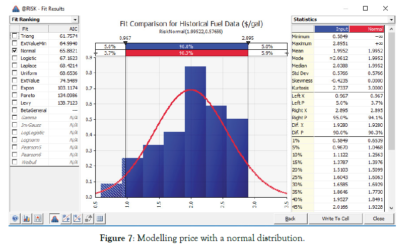
Figure 6: Modelling price with a normal distribution.
Caution – the Normal distribution has tails that go in both directions to infinity. By using the normal distribution as our model this will result in unacceptable values for the price (negative values and extremely high numbers). Limiting the extreme values to some boundary (i.e., 50 cents and $3.50) might make sense. This is especially important if your model is an input into other simulations.
Appendix 2: Explanation of triangle distribution fit for demand data
Sometimes there is no data available. If this is the case, a common modelling technique includes eliciting modelling information from subject matter experts (SME’s). This could result in the following exchange: The lowest demand that our organization has ever had is 75k gallons and the highest demand is 127k gallons. Additionally, our most likely demand is something close to 100k gallons per year. With this information, you can directly input a triangle distribution into @RISK to represent the demand. It would look like this: =Risk Triangle (75000, 100000, 127, Risk Name ("Demand Data (gal/year)").
Since we have data, we could utilize the 36 data points for demand, and model demand behavior by highlighting the demand data and clicking on “Distribution Fitting” in @RISK. By selecting the Triangle Distribution and deselecting all other distributions, we have chosen a model and written this choice to a cell that now represents the uncertainty of demand. Figure y is the resulting model (Figure 7).
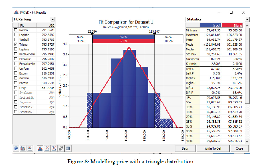
Figure 7: Modelling price with a triangle distribution.
Notice the parameters for this fitted distribution (75088, 101628, 126823) are very close to what our SME’s provided (75k,100k,127k). That may not always be the case, and, a sound analytical process should review assumptions by comparing them to ‘real world’ data as part of the model verification and validation process. Also note the Triangular distribution is bounded on both ends, which mitigates problems encountered using a Normal distribution (i.e. with tails from positive to negative infinity).
Appendix 3: Putting it all together – simulation model for annual fuel costs
Using a Normal probability distribution as our model for Price and a Triangular probability distribution as our model for the Requirement (Quantity), we complete our model by simply multiplying these values together to get an annual budget estimate that captures the variability of both price and demand. After designating a cell as the output cell in @RISK and running our simulation model 5000 times, Figure z is our output (Figure 8).
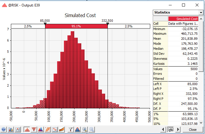
Figure 8: Modelling an annual budget as the product of price and demand.
Note: Extreme values, such as the minimum value for this simulation of -32076.15 and maximum of $460,000, are often meaningless. In this case, they are simply artifacts of using a normal probability distribution to model prices (with tails from negative to positive infinity). Budgets in the bulk of the probability area captured through confidence intervals are the only values of interest for our guess estimation.
Citation: Melese F (2021) A Data Analytic Guide for Defence Management and Budgeting. J Def Manag. 11:5.214.
Received: 27-Jul-2021 Accepted: 16-Aug-2021 Published: 23-Aug-2021 , DOI: 10.35248/2167-0374.21.11.214
Copyright: © 2021 Melese F. This is an open access article distributed under the term of the Creative Commons Attribution License, which permits unrestricted use, distribution, and reproduction in any medium, provided the original work is properly cited.