Mathematica Eterna
Open Access
ISSN: 1314-3344
ISSN: 1314-3344
Mini Review - (2024)Volume 14, Issue 3
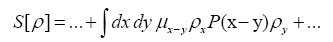
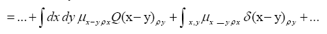
This article presents the mathematical foundation for calculating PD's (Probability Distributions) for some set of phases {ϕh} needed for the structure determination of a crystal. We can obtain PD's of the phases that can contain N or without N. A former paper could only obtain PD's of the phases containing N. Here we have the two possibilities.
Random variable; Reciprocal vectors; Binomial distribution; Infinite number; Phase
In a short review was given of the old probabilistic DM (Direct Methods) way for calculating phase distributions [1].
There were two mathematical approaches see (A) and (B) below
(A): The basic R.V.’s (Random Variables) are the set of the  that are distributed independently and uniformly over the asymmetric unit (we consider in this paper only P1) and one studies the normalized structure factors
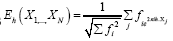 And one calculates the probabilities of the phases
 (B): The basic R.V.’s are the reciprocal vectors h that are distributed uniformly and independently over reciprocal space and one keeps the Xiconstant. This method can give algebraic equations as follows: One can study the structure factors
 and we consider only h as the basic reciprocal vector and one keeps k fixed. The B3,0 formula is an equation obtained this way. Although this equation gives the value of
 in theory, in practice this equation is wrong for high N, which is due to accidental overlap of the xi which invalidates the calculation of the joint probabilities of
 Even when one calculates the joint probabilities
 where h and k are the basic R.V.’s one must assume no accidental overlap of the xi (which becomes a problem for high N.). The calculation of joint probabilities gives then the same results as in (A) above.
(C): Using method (A) one can derive the probability of the cosine invariant

It follows that this formula
Loses predictive power for high N.
Cannot predict negative cosines.
The probabilities of quartets, quintets, etc. are even worse since they are of order of 1/N (for quartets), of order (for quintets), etc. (Although one can get a quartet formula that theoretically predicts negative cosines for the quartet (but again with too low predictive power)). At the end of the twentieth century nobody was busy anymore with calculating prob-abilistic phase distributions using one of the methods (A) or (B). For the calculations of structures with high N (N being here the number of independent non-H atoms in the asymmetric unit), one began to devise methods in direct space to solve crystal structures. One uses an automatic cyclical process: (a): Phase refinement (for instance with the use of the (modified) tangent formula) in reciprocal space and; (b): With the imposition in real space of physically meaningful constraints through an atomic interpretation of the electron density, with minimization of a well-chosen FOM (Figure Of Merit) of the phases. One of these methods in DM is known as the SnB (Shake and Bake) algorithm with N 1200 [2,3]; Another is the twin variables approach with
 Sir2000 the successor of SIR97 and SIR99 although different from SnB: (e.g. triplet invariants via the P10 formula with
 Another interesting result is the solution of a crystal when a substructure is known where N may become higher [4-9]. For an overview of DM before the year 2000 we refer to Giacovazzo [10].
(D): In order to circumvent these problems one approach might be to consider R.V.’s (xi)that are no longer independent neither uniformly distributed, say a dependence through a positive distribution
One can give such distributions by using the functions 
But then one encounters insurmountable mathematical difficulties.
The solution is to not consider the xi as R.V.’s anymore but to replace by a field
 and to sample the field over the allowable function space. What we shall discuss here is a novel way for doing DM (Direct Methods).
(E): Differences with our approach
• We shall be able to solve any structure (any N) ab initio.
• Much lower CPU time.
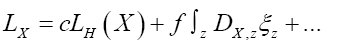
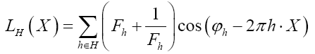
• Let then with our approach we can easily calculate the probability distribution of
 for any h. No need to compute all possible triplets.
• Easy to incorporate any given substructure.
• Easy to calculate the PD’s (Probability Distributions) of phases: One only needs to take derivatives.
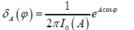
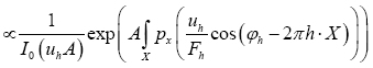
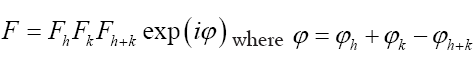
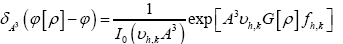
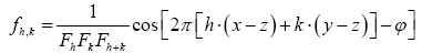
In this paper we shall give the mathematical basis that is necessary for this completely new DM approach. This approach is not mathematically as simple as in (A) and (B) but it is perfectly doable. It consists in using the atomic distribution function (x) as the basic random variable. The method will also be based on a functional integration over the random variable and using a nonstandard fuzzy approach wherein Dirac delta functions (among which a novel delta function representation for angle variables) are replaced by nonstandard fuzzy delta functions. To show the strength of the method, a simple formula was given in Brosius for the distribution of the triplet phase formula of the form 
Where A is a function depending (not on N!) on the structure factors of the first neighborhood of the triplet [1].
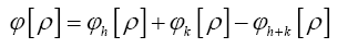
In this paper a more profound mathematical foundation of our DM approach is given and this will be a major improvement compared to Brosius [1]. Recall that the sampling is done over positive functions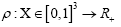 (in the space group P1) and that the R.V.’s that we study are the phases
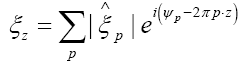
  which are defined by the relation
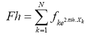
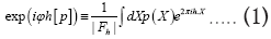 Where is a R.V. defined by
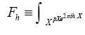
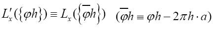
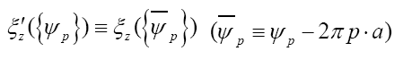
and from now on we shall use the notations

One then needs to define a probability density  on the sample space ρ's We build up by fuzzy Dirac delta functions in 4 steps
Through constraints of the form  by using fuzzy Dirac delta’s
  (εa positive infinitesimal).
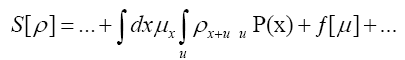
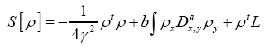
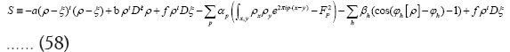
Next through maximization: Adding obvious terms to where
where that cannot be added by using a constraint, like e.g. the term.
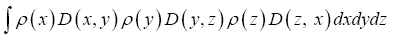
Eventually we add fermionic terms to z, like e.g.

By imposing the mathematical requirement on the basic R.V. ρ that the different atoms in the unit cell of the crystal repel each other.
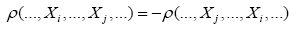
The idea is that if one would consider a function 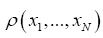 for which it is known that
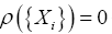 whenever xi equals some xj, this can be done by requiring that
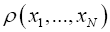 is antisymmetric antisymmetric xi, that is
Inspired by modern QFT (Quantum Field Theory) we replace  by an antisymmetric (fermionic) field
  with the property
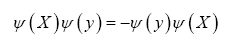
giving thus

The added benefit is then that the different xi will repel each other. Now one has two basic R.V.’s: ρ and ψ and we must integrate over ρ and ψ.
One can also sample over the set of Gaussian (normal) distributions by using the substitution
where  represents the true electronic distribution and
  is the laplacian of f at the point x.
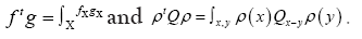
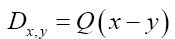
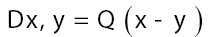
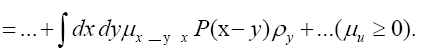
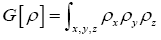
As in QFT, D (x, y) is called the propagator from the point y to x. Using constraints we shall see that the first candidate for D (x,y) is Q(x–y) where Q is the origin-removed Patterson function defined here by
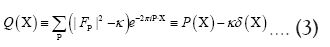
This propagator depends on N since 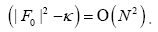
Notations and formulas

A without subscript stands for some infinite positive number.
 where
where is the inverse of the kernel operator Q(x–y)
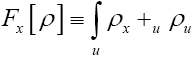
The phase random variable  is defined by
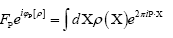 where
where denotes the atomic distribution and the function ρ is our basic R.V.
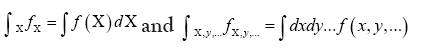
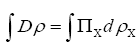
The functional integral
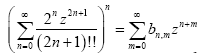
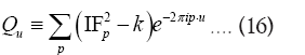
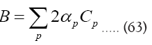
The  constants. We define the constants by the series

The bn;m constants, defined by
Our representation of  for an angle
 is
is
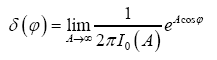
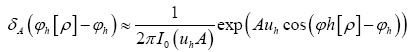
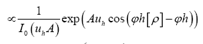
We then define the fuzzy nonstandard  function by
For real x (not an angle) we define the nonstandard fuzzy by
by
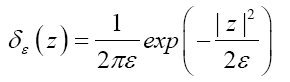
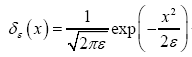 for positive infinitesimal ε, and for complex
For some set H of reciprocal vectors we define
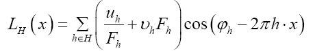
and sometimes we simply write 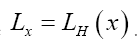
We use the explicit definition of the functional derivative by
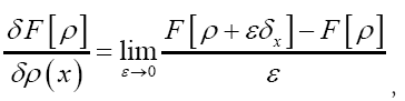
Where
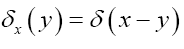
where 
 ; Where
Some vector calculus: (f, g: vector valued functions, h a scalar function)


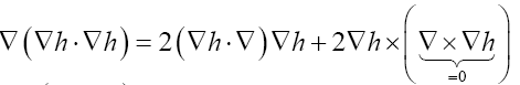
Recall that in three dimensions
Preliminary knowledge
For an introduction on nonstandard theory we refer to Diener et al. and for a more advanced text see Nelson [13,14].
Nonstandard theory: Standard numbers are the known numbers:  the other numbers are the nonstandard real numbers which make up the field R. It is important to observe that there are an infinity of infinite numbers in R that are greater than any standard real number. Also there are an infinity of infinitesimals ε in R for which the absolute value |ε| is less than any positive standard number in R. From the axioms it follows that for every positive infinitesimal
 is a positive infinite number and vice versa. Note that an infinite number is different from
 In this paper we use A to denote an infinite positive number and ε will always denote (unless explicitly noted otherwise) a positive infinitesimal
  will denote a function that associates a positive infinitesimal with every position x in the unit cell
 We will use this function in our fuzzy Dirac delta.
 We shall use the notation
 when we deal with angle variables.
Anticommuting variables: In a detailed exposition of anticommuting numbers is given [1]. In this subsection we shall only expose the bare minimum needed to read this paper. For more information, we refer to Weinberg, Siegel, Kuzenko et al. and for a more mathematical treatment to Bruhat et al. and deWitt [15-19].
One starts with a set of anticommuting numbers θλ:
From this follows that every even product of such anticommuting numbers is commuting Also one adds the axiom:
 Then the algebra
 is defined as the set of all finite sums of products.
When M is even, this is a commuting number (also called even) and when it is odd it is an anticommuting number (also called odd). Sums of such products with even M do commute and are called even, and with odd M these sums are anticommuting and are called odd. Every z∈C is also even. It follows that every  is a sum
 with β even and γ odd.
An involution  defined such that,
  and
and
 is odd when
 is odd and even when otherwise. One calls
 is odd when α is odd and even when otherwise. One calls ψ or ψx an odd function of x if ψx is odd for every x. It then follows that
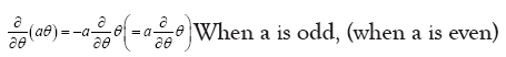
 is even. Then the derivative
 with respect to the anticommuting variable θ is defined by
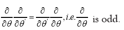

 where
where
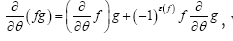
A function  of an odd variable θ has the simple form
 (Taylor expansion), (here a is odd when f is odd, and even otherwise, but b has the opposite statistics of f). This can be generalized for a function
 of N anti-commuting variables: The coefficients of even products in the expansion of the θi have the same statistics as f, whereas the coefficients of uneven products have the opposite statistics. Next one defines the integration
 as
as
and the multiple integration
It is also convenient to define θ as an odd element:
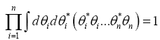
Also the following formulas are important
Note that the set of all odd numbers has vanishing volume
 and
and

The four determinants are listed below. The following Theoremes are:
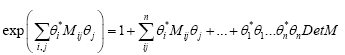
Theorem 1: Let M be an matrix n×n– matrix. Then
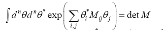
where by definition 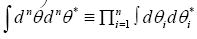
Proof develop 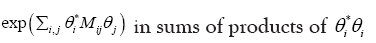
Since,
 the theorem follows.
The continuous version is as follows. Let be an anticommuting variable for every X in the unit cell. Then,

where one has defined 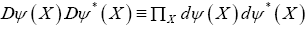
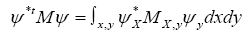
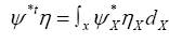
Theorem 2: Suppose now that the inverse M–1 exists and be an anticommuting variable for every X. Then
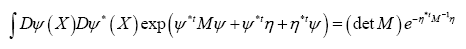
Where
Proof let
Then transform
and substitute this in  Then using the relation
Thus
Also

The minus sign arises from the observation that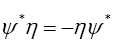 in
in
Indeed, note that
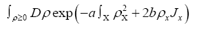
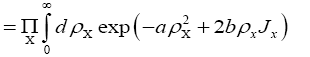
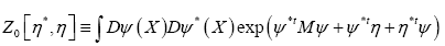
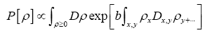
The probability functional
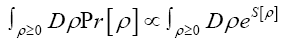
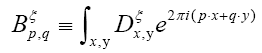
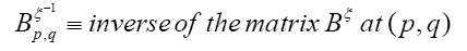
We shall show that we can obtain the following probability function 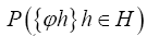 (H is some set of reciprocal vectors) given by
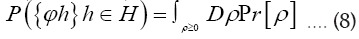
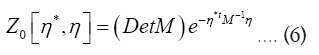
where  is given, up to a phase unimportant constant, by
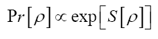

where  denotes chemical information or an intermediate iteration of ρ.
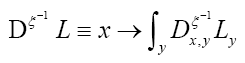
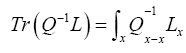
 will be the basic operator for all our
 First we need the following theorem:
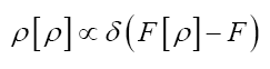
Theorem 3: Let be a functional of
  such that
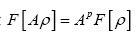 where A is a positive infinite number and p an integer ≥1. If we impose the constraint
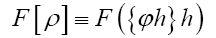
where F has the property that 
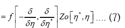
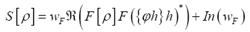
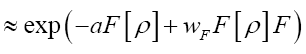
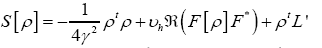
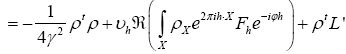
Then if we define the action functional 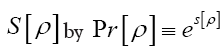 (where c>0 is a constant) Then
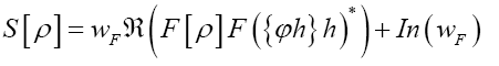 (where wF>…. (10)
For a sequence of such  will become (if we drop the constant
Proof we impose this constraint by 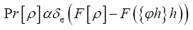
Since  is independent of the ϕ,h one can drop it in the above exponent. Next change
 and choose
 Since
Since one obtains
since  (infinitesimal). Also under the change
 integral volume
 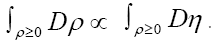 So finally ( after replacing
 (if we drop the constant
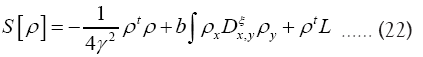
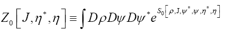
Theorem 4:One can write 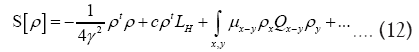
Where
where from now on  is included
  convenience, with parameters
Proof.
 and use the Dirac
 Then
Then


where we defined  such that
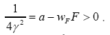
• The R.V.  was defined by
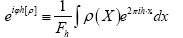
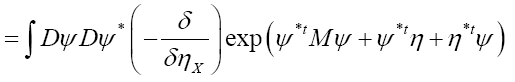
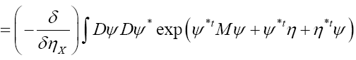
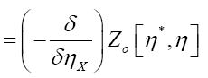
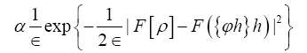
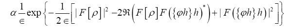
Then the probability distribution of  is generated by the expression
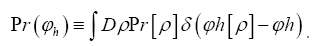
But, (when A is infinite and positive)
After the transformation 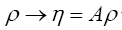 obtain the result
where 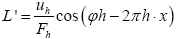 For convenience, from now on, we shall include
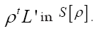
• Next use 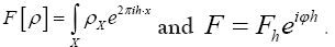 Then
Then
where 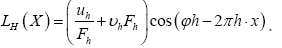
• For every  we impose the constraint
where
and
Then, according to theorem 1 above, one has
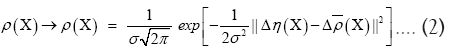
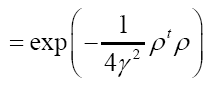
Next note that there is a phase unimportant peak  and define Q by
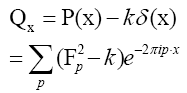
Then if one chooses the positive function 
One can also add other terms to  For example consider the triplet expression
Impose now the constraint  Since
Since and
and is constant in the phases we can write according to the basic theorem
where  One can also do the same for quartets, quintets and so on. Next impose for the triplet, the constraint.
where

Note that Important, 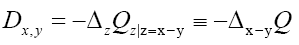 from now on we shall treat all weights
 the same: We shall not distinguish between the different measurements
The same will be true for  The same is true for the
  But we shall not consider triplet terms of order
 in this paper. So now we have arrived at
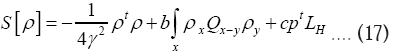
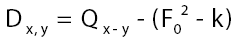
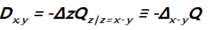
This propagator Dx,y does not depend anymore on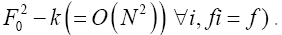 In the sequel we shall simply say: “does not depend anymore on N”. It is better than
 Indeed to see this we can write
 as
as
This last expression becomes very low whenever x-y is not an interatomic vector since then  and thus
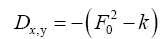 and thus
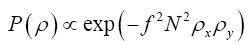

That is  demoting such a ρ. We recall that we have also
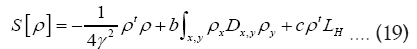
Recall that 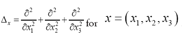 In order to see what this new propagator can offer let us look at Qx.
Qx is an N-sum of gaussian functions. Let us consider one of them, say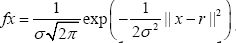 For sake of convenience we take now
 and we consider the one dimensional case
 Then
Then And
And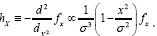 Thus at x=0 we see that
 times larger than
 since
since which is very large since σ is very small. The function
 then drops very fast to zero at
 after which it remains negative, attains a negative minimum and then goes fast to
 Also there is exactly one large negative minimum in the range
 Exactly as discussed
 for a ρ for which
  at one of these minima. For
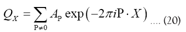
we get 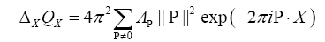 Because of the differentiation
 this
this  does not depend on N
Note, 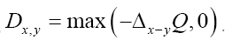 This
This can also be used; Then there are no negative minima, but in order to make it N independent, one has to follow the procedure used in
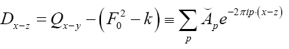
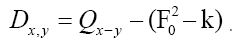 That is we must subtract the term
 in the Fourier expansion of
  to get a new propagator that is N-independent:
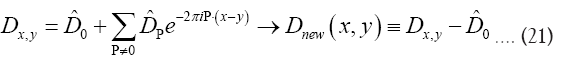
Improvements 
Let d be the maximum distance of all  where
where is the nearest neighbour of
 Then we can obviously replace the
 is the characteristic function of the sphere
 in the asymmetric unit of the crystal. Thus
 becomes
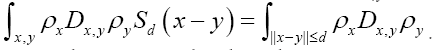 If we know d we can then improve the phase densi- ties
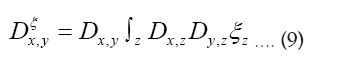
 When ξ is a given chemical information (be it a submodel or an intermediate state ofduring iteration) then we can derive a new propagator, with notation
 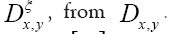 Indeed if we look at the term
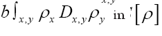 it is clear that we can consider an (improved) term
 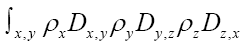 and replace
 with the latter term. For instance if
  when and
 and
and  are interatomic vectors; This is a stronger restriction on than merely the condition
 Now if
 is a submodel of then we can also replace
and obtain again a term of order  by replacing
 by the stronger condition (on ρ )
 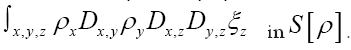 But now also
 changes to
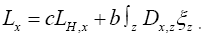 Indeed, in
 we can replace
 Then
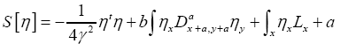
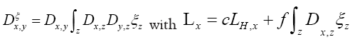
Then becomes
  where now
  (Remark that
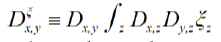 is symmetric whenever
  and we replace b by another parameter f. Hence for a given submodel ξ we can now write a better
with 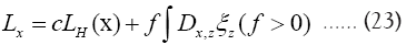
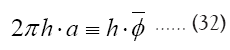
Example: We can always place the origin of the asymmetric unit wherever we want, i.e. we can always suppose that one atomic vector, say a, is given. This means that at least we can always use the chemical information. 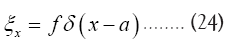 Then we get
Now we can show that with this we can directly calculate the density of the phase invariant.
 instead of simply
 Indeed consider the functional (where we
Next we do the functional change of variables:  where
where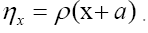 Then the Jacobian is the inverse of the determinant of the matrix
 which is not dependent
 Then
Then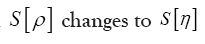
and 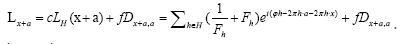 Defining the phase invariant
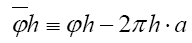
and considering the case that interests us most 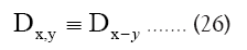 we can write now
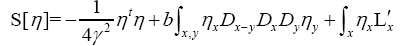
Where now 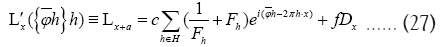
Remark: is indeed a phase invariant because under a translation of the origin
 also
also and thus
 under this translation which shows that
 is indeed a phase invariant. For the reciprocal vectors
 we can write
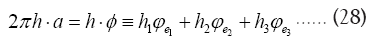 where
where So we can write the phase invariant
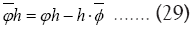
The case for general ξ: Let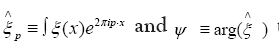 then
then 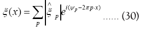 and consider
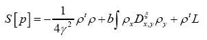
 Then we apply the same functional change
 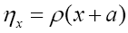 and we then get for
where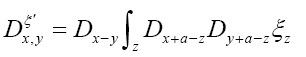
Note: From now on we shall always write 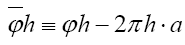 instead of
 instead of
 resp.
resp. 
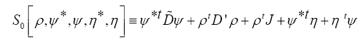
A fermionic action functional and a new
One knows that the different atoms in the unit cell repel each other. So, our random variable ρ should be chosen in such a way that the different peaks of ρ(x) spread over the unit cell and repel each other. This can be treated by considering ρ as an antisymmetric (fermionic) field written now as ψ. Then, following the treatment of QFT (Quantum Field Theory) [15], we replace.
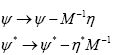
Remark that will be replaced by
  which must be even and hermitian. So
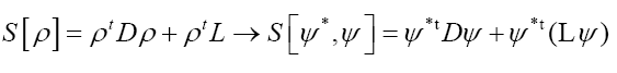
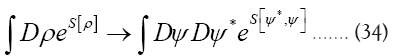
Next 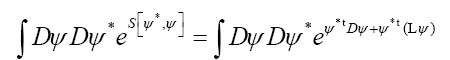
where I is the identity operator and we now replace 
We then get (where is the inverse of the operator
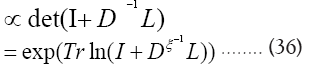
since det  does not depend on the and since
 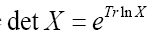 for a matrix
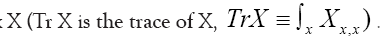
We can write
Then using 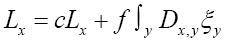

A fermionic action functional and a new
Since 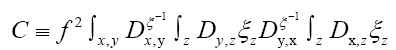 does not depend on the
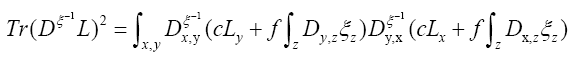
we can dismiss it in equation (38). Next continue with the case and
and and we define
Then for 
To get some idea let’s consider the simpler case 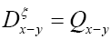 but still
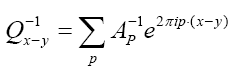
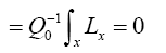
Then the inverse of Q, i.e. Q-1reads
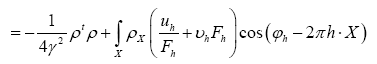
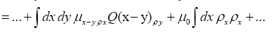
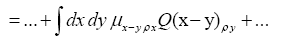
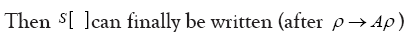
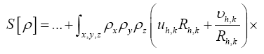
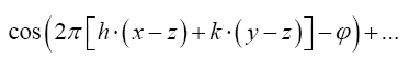
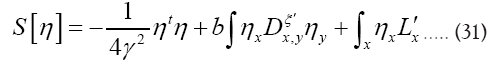
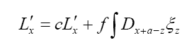
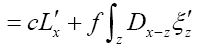
Then
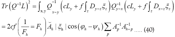
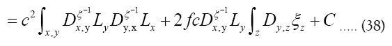
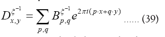
Where we omitted a term in equation (40) that does not depend on ϕh. In equation (40) we have used the identities

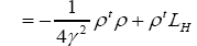
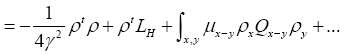
Finally, for 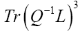 we get (omitting the terms that don’t depend on

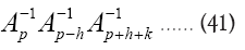
The terms 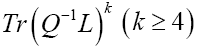 are of higher order in f and c. So we see that we obtain in this way a probability of the form
 and thus
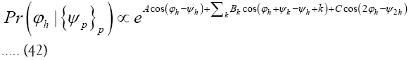
Equation (41) shows that for this model it is advantageous to choose f=c and then to use c for convergence considerations. For example, Equation (42) is then valid up to 
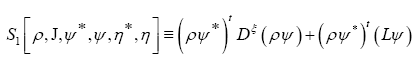
We can extend the above model and study instead the model with action.

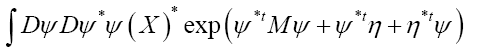
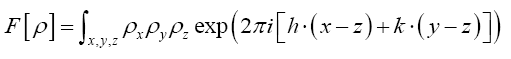
To calculate then the functional integral  we use the following trick.
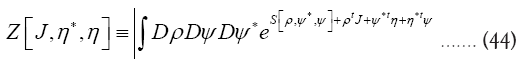
If we then define
Then
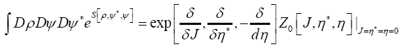
where the choice is clear and where we choose
 and invertible to make calculations easier
  Let us define
The it can be shown that  contains exactly all the connected diagrams of
  [1,15,16]. It is beyond the scope of this article to talk more about diagrams, but we shall discuss it together with the solution in a future paper.
Averaging over gaussian distributions ρ
So far we have been averaging over all positive  But what if we want to average only over gaussian ρ functions? The solution is the functional change of variables
 where
where is the true atomic distribution; This substitution is good if we don’t care about N-dependence, if we don’t want N-dependence we should instead consider
That is 
where  is a positive function, our new random variable.
Since  and thus also
  is about the true density they are completely determined by the phases
 In this way we will get a probability distribution of all
 Then the “volume” element
  , that is
This can be calculated but we can avoid this added complexity if we remark that we could have started from the very beginning by using instead of ρ the more complex form that is we replace
 and so on. Replacing next the symbol
 by
by  we then get
 etc. In this way the former is now describing “point” particles. However, the whole use of functional integrals in QFT is to describe interactions among point particles. So we do not know if it is worth doing averages over those Gaussian “point” particles.
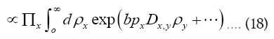
We close this remark by giving two representations of the δ function. One is to represent by a gaussian with infinitesimal variance. The other very interesting representation is
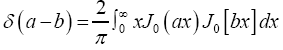 In our case it reads
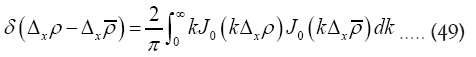
We can then first integrate over ρ and after that perform the integration over k, which is much easier.
Maximality with constraints
We saw in the foregoing sections that we had to maximize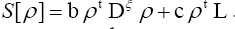 Let us analyze this further. We shall now start with
 We will maximize this with the constraints
 for all
 Next observe that
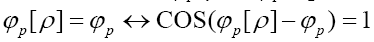 We then use the method of Langrangian multipliers. Put now
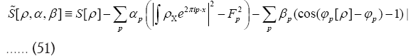
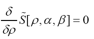
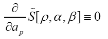
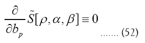
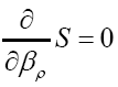
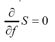
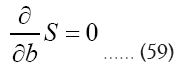
The minus signs in equation (51) have been chosen so as to use later on the more general “KKT- multipliers”) and find the solutions 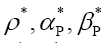 for which
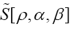 is maximal (critical), that is solve the equations
Next
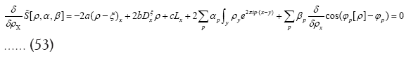
Next observe that
Since  has now become redundant, we replace
 in equation (51). We can also add inequality constraints for ρ


and
In this case the multipliers  multipliers (KKT stands for Karush- Kuhn-Tucker). And we have a dependence
 now on
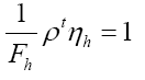
It follows from the above equation that we can impose (we suppose in this paper that friedel’s law is valid, that is  and
and

We use the notation to denote the transpose of A, and then
 We have to solve


We find
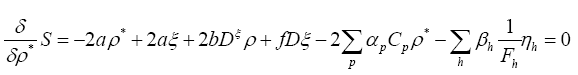
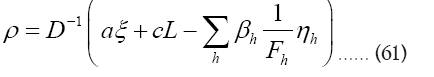
This gives (using ρ* instead of ρ)

and thus
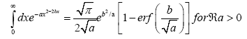
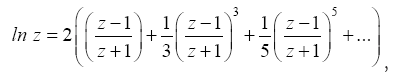
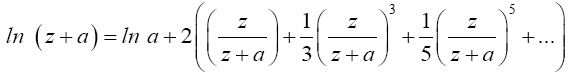
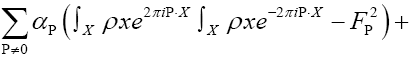
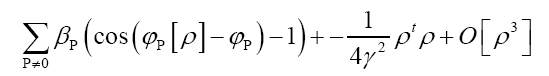
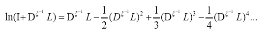
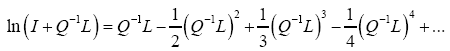
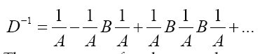
Next we develop [16]
[16]
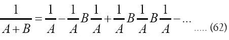
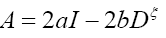
Then,
Then we can write if we choose a to be great and b small (a>>b)
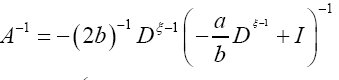

or if we choose a small and 
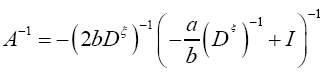
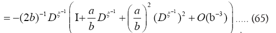
Since we prefer to use the easier  instead of
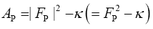
 we shall in this paper proceed with the development of equation (64). Then for a>>b we find
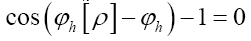
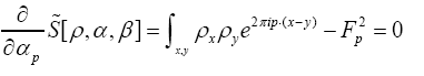
Next 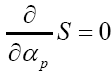 will give
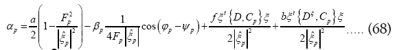
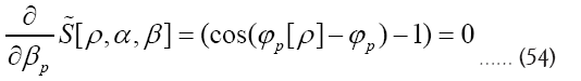
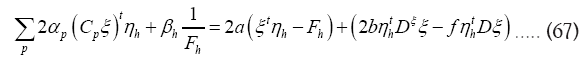
From  follows
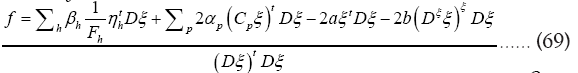
From the equations (67,68) we derive the values of αp and βp as functions of f and b. From these results and equation (69) we derive the value of f as a function b. We now see that are of order
  . If we would derive the value for b with the condition
  then we will also see that b is of order which gives a problem since we started with the assumption (a>>b)
For this reason, we shall not impose the condition The bare minimum is the calculation of all the Lagrange multipliers
 and one or more Lagrange multipliers
 All the multipliers depend strongly on the phase invariants
 The situation becomes even more interesting if one now calculates
 and this is good news. We think that this last model is very exciting (perhaps it can even be used to construct the exact ρ from any given ξ). We will study all this in a separate paper.Now
  can be written in a short way as
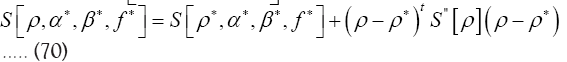
Since  and moreover one can verify easily that
 is a constant in ρ.
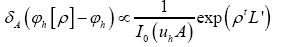
To calculate a probability distribution prob  for some phase
  one chooses one of the models discussed in this paper and also some
  of reciprocal vectors containing h. Then one calculates
 according to the chosen model. After that one calculates the marginal distribution
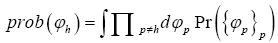 Always choose structural information ξ e.g. the fixing of the origin
 All models should lead to the solution of the phase problem.
In a future paper (II) we shall study in detail all different models but especially the fermionic model and the one of maximality with constraints. Especially we shall discuss the most general fermionic model and we shall talk about the technique of the diagrams to calculate
For the very interesting model of maximality with constraints we shall also add the KKT condition  with some KKT multiplier
 Finally, in a last paper (III or IV) we shall test the theory on simulated crystal structures.
We shall also discuss which strategy to use in case of available space group information. Our paper treated only the space P1 (satisfying Friedel’s law). Our use of functional integration and calculus is much more powerful than the other methods of phase determination, be it probabilistic or direct space methods and is valid for any number N of atoms. We shall also try to discuss models for which the formulas will depend N.
[Crossref] [Google Scholar] [PubMed]
[Crossref] [Google Scholar] [PubMed]
[Crossref] [Google Scholar] [PubMed]
[Crossref] [Google Scholar] [PubMed]
[Crossref] [Google Scholar] [PubMed]
[Crossref]
Citation: Brosius J, Brosius W (2024) Probability Distributions of Phases I. Math Eter. 14:226.
Received: 11-Jun-2024, Manuscript No. ME-24-31944 ; Editor assigned: 14-Jun-2024, Pre QC No. ME-24-31944 (PQ); Reviewed: 01-Jul-2024, QC No. ME-24-31944 ; Revised: 08-Jul-2024, Manuscript No. ME-24-31944 (R); Published: 15-Jul-2024 , DOI: 10.35248/1314-3344.24.14.226
Copyright: © 2024 Brosius J, et al. This is an open-access article distributed under the terms of the Creative Commons Attribution License, which permits unrestricted use, distribution, and reproduction in any medium, provided the original author and source are credited.
 [
[