Mathematica Eterna
Open Access

Pricing Gamma based Temperature Derivatives

Kondwani Daniel Vwalika^{* *}Correspondence: Kondwani Daniel Vwalika, Department of Mathematical Science, University of Malawi, Zomba, Malawi, Email:

Author info »

Introduction

Temperature plays a vital role in agricultural growth and production, impacting crop development, seed germination, flowering and fruit ripening. Extreme temperatures, whether too high or too low, can adversely affect crop yields and quality, causing heat stress, reduced photosynthesis, water loss, slowed growth, frost damage and diminished pest control effectiveness. To mitigate temperature-related risks, various approaches are employed, including irrigation, breeding for heat and drought tolerance and the use of shade nets and greenhouses. An emerging and popular method for risk management is the use of weather derivatives financial contracts linked to specific weather events or indices. These derivatives offer advantages over traditional insurance, being more cost-effective, flexible and transparent, based on objective weather data. The weather derivatives market has seen significant growth since its inception in 1996, primarily driven by the energy sector in developed countries. In developing countries, weather derivatives are gradually gaining traction, especially in agricultural and renewable energy sectors. However, challenges remain, such as the lack of standardized weather data and regulatory barriers. Call options are more commonly used in developing countries for weather hedging due to their simplicity and accessibility. The study aims to price weather derivatives using data from Chitedze research station, providing coverage for farmers against unfavorable temperature conditions and ensuring payout security.

The majority of authors who employ the Ornstein-Uhlenbeck (OU) model assume that the noise follows Gaussian Wiener, Levy or fractional Brownian motion, as noted by Dzupire et al. Using the first two processes implies independent temperature changes, but authors note correlations in changes. Temperature reverts to seasonal trend, confirming the argument. Meanreverting parameter captures this behavior. Certain researchers utilize fractional Brownian motion as an alternative to assuming independence. However, it remains uncertain whether the issue is completely resolved.

It is reasonable to assume independence in the random noise process while still retaining the characteristic of reverting to the regular trend. Nonetheless, it is justifiable to consider temperature as Markovian, implying that the mean-reversion parameter should encompass autocorrelation. The authors highlight that this parameter reflects the rate at which temperature returns to its seasonal average. The question not answered by many authors is how to ensure that this parameter also captures information about autocorrelation. Additionally, using the Ornstein-Uhlenbeck (OU) process implies the underlying probability distribution of temperature follows a Gaussian family, like the normal or inverse one.

The Kolmogorov forward equation (Fokker-Planck equation) can be satisfied to acquire the particular probability distribution resulting from the fitting of the OU differential equation. Satisfying these additional partial differential equations addresses nonlinearity and non-stationarity problems, emphasizing the Gaussian family probability distribution. Nonetheless, historical temperature datasets frequently exhibit deviations from a normal distribution. This discrepancy has prompted authors to utilize the normal inverse Gaussian distribution in order to depict data that displays skewness and possesses heavy-tailed characteristics [1].

The gamma distribution, a widely used probability distribution for modeling weather variables, such as rainfall, evaporation and temperature, has two parameters (shape and scale) that can be estimated from historical temperature data. Modeling temperature using the gamma distribution helps estimate the likelihood of extreme temperature events and corresponding financial losses, which is relevant for pricing temperature derivatives like call options. While the gamma distribution has been used to model temperature, its application to weather derivatives remains less explored.

Several studies have used the gamma distribution as a flexible and accurate model for temperature. For instance, Andrews and Shivamoggi [2], found the gamma distribution provided a good fit to temperature data and effectively estimated temperature, while Moriarty et al. [3], found it suitable for estimating expected temperature in the future. Haddad [4], shows the gamma distribution is appropriate for daily temperature readings, accommodating both maximum and minimum temperatures and non-negative values. However, the literature does not address how to ensure an associated stochastic differential equation satisfies the Fokker Planck equation and Markovian auto-correlation. Stochastic Differential Equations (SDEs) are widely used mathematical models in various fields such as physics, finance and engineering, derived through methods dependent on stochastic calculus type or moments.

Three techniques for deriving diffusion time evolution are commonly utilised. The first is Ito calculus, based on the Ito formula, which defines SDEs using underlying physical or economic processes and is widely used in finance and economics. The second is the Stratonovich calculus, similar to Ito calculus but with a different interpretation of drift and diffusion terms, often applied in physics and engineering. The third is the Fokker-Planck equation, a partial differential equation describing the evolution of the probability density function of a stochastic process, useful for studying long-term behavior. However, converting partial differential equations into SDEs can result in information loss. Another approach is the method of moments, which involves finding moments like mean and covariance from SDEs, derived based on physical intuition, data analysis and domain knowledge. However, this method relies on assumptions of stationary moments and independence, which may not be valid in some cases.

The Kalman filter [5], is a widely used recursive algorithm in stochastic control theory and engineering that estimates the system state based on measurements and a model. However, its numeric drift and diffusion coefficients make it challenging to incorporate temperature data’s seasonality. To address this, the Bayesian estimation method utilizes Bayes’ theorem to update probabilities of system states, commonly employed in decision making and machine learning.

Nevertheless, recurrent neural networks require large sample sizes for accurate seasonality capture. Existing methods fail to ensure that differential equations capture nonlinearity, nonstationarity and auto-correlation in data. To address this, Primak et al., introduced a synthesis method for deriving Ito’s stochastic differential equations, satisfying Fokker-Planck equation and auto-correlation intervals, commonly used in telecommunication and non-seasonal data. This study intends to use the method to derive stochastic differential equations for seasonal temperature data.

Weather derivative pricing commonly involves Esscher transforms, stochastic optimization and discounting expected payoff [6]. The reflection method, constructing Brownian motion from temperature and reflecting it to estimate prices, is difficult to incorporate temperature readings in Brownian motion noise.

Esscher transform uses probability density to price derivatives but may lose time-dependent parameters. Geman and Yor [7], proposed a Brownian motion-based equilibrium approach for pricing temperature derivatives, extending the model with stochastic volatility for heating degree day options using Monte Carlo simulation. Scher and Messori examined temperature forecast uncertainty’s impact on weather derivative pricing, proposing a model incorporating both forecast uncertainty and temperature volatility, although lacking the most accurate pricing. Hess [8], introduced a forward-looking weather model for pricing rainfall derivatives, showing improved accuracy over models ignoring rainfall-temperature correlation.

Ahčan [9], proposed a new model using the variance gamma process for pricing temperature derivatives, capable of pricing both heating and cooling degree day options but with weak estimations. Another early model is the Seasonal Autoregressive Integrated Moving Average (SARIMA) introduced by Liu et al. [10], effective for pricing simple temperature derivatives like Heating Degree Day (HDD) and Cooling Degree Day (CDD) swaps, capturing seasonality and long-term trends. Another approach is using the Ornstein-Uhlenbeck (OU) process, introduced by Zhu and Bauer, which is a mean-reverting process suitable for pricing complex temperature derivatives, including HDD and CDD swap options. Additionally, other proposed models for temperature derivatives pricing include the Regime- Switching model (RS), allowing changes in statistical properties over time, the Jump-Diffusion model (JD) capturing sudden jumps in temperature data and the Stochastic Volatility model (SV) handling temperature data volatility.

Pricing temperature derivatives remains challenging in finance, with model choice depending on temperature data characteristics and derivative complexity. Ongoing research aims to enhance accuracy in temperature derivative pricing models. Alaton et al. [11], applied martingale methods to value weather call options; however, this approach contradicts the Black- Scholes assumption of market completeness due to the nontradability of temperature. This study uses the method of discounting expected payoff, incorporating temperature model information and probability density [12].

In summary, the existing literature has extensively explored the development of a more precise and efficient stochastic model for temperature forecasting, aiming to enhance the pricing of weather derivatives. However, the potential of the derived stochastic model for forecasting temperature values remains unaddressed in the literature. Furthermore, there is a lack of research on how the derived stochastic model can be utilized to price temperature derivatives effectively. Additionally, the literature has not provided a comprehensive understanding of how the mean-reverting Ornstein-Uhlenbeck (OU) process, employed by Scher and Messori, Hess and Zapranis and Alexandridis, tackles non-linearity and non-stationarity in temperature data through the satisfaction of the Fokker-Planck equation. Specifically, the limitations of the OU process in dealing with autocorrelation intervals in temperature data remain unexplored. Therefore, it is crucial to investigate how the proposed stochastic model can be constructed to incorporate autocorrelation interval parameters in both diffusion and drift components, enabling it to effectively capture autocorrelation, nonlinearity and non-stationarity in temperature data. This endeavor will provide insights into how the inclusion of autocorrelation interval parameters in the proposed model enhances the accuracy of temperature predictions.

Materials and Methods

To solve this problem, this paper derives a stochastic model from temperature that follows a gamma distribution. By utilizing the synthesis method for deriving diffusion and drift coefficients, we incorporate a parameter representing the autocorrelation interval in the model. The satisfaction of the Fokker-Planck equation enables the parameters to capture nonlinearity and non-stationarity in the data, resulting in more accurate daily temperature predictions. With this model, we can predict temperature values that are subsequently used to estimate prices of gamma weather derivatives, whose underlying asset is temperature.

Preliminary concepts

Gamma distribution was fitted to daily temperature data. Below is the provided description of the gamma distribution as outlined in the work by Haddad [4].

Definition 1: A gamma distribution is defined for a random variable Y when its probability density function is expressed in the following manner.

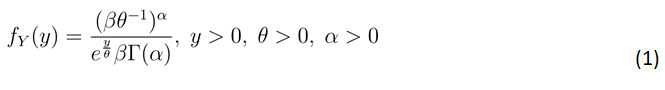
When value of Γ (α) is determined as follows:

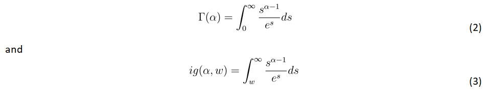
The term used to denote this concept is referred to as the upper incomplete gamma.

Lemma 1: lim_α→∞ Γ(α)=∞, lim_α→∞ ig(α,w)=∞ and lim_w→0 ig(α,w)=Γ(α)

The significance of this lemma is that when applying gamma distributions to model temperature, it’s important for the α values to be moderate in size. Furthermore, if the w values are small, employing the gamma function is also a viable option.

Lemma 2: If Y follows gamma probability distribution with parameters α and θ, then the mean of Y is given b,

E(Y)=αθ

its second moment is given by

E(Y²)=αθ²(Α+1)

and its variance is

Var(Y)=αθ²

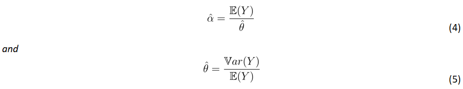
Definition 2: The method of moment estimators of the parameters α and θ are given by

This study focuses on univariate stochastic differential equations of Ito’s type to model temperature given that it follows gamma distribution.

Definition 3: Ito’s stochastic differential equation is given by

dY_t=μ(Y_t,t)dt+σ(Y_t,t)dW_t (6)

μ(Y_t,t) is the drift coefficient, σ(Y_t,t) is the diffusion coefficient

Definition 4: W_t is the standard Brownian motion and is defined as the stochastic process {W(t),t ≥ 0} such that P(W(0)=0)=1, E(W(t))=0, Var(W(t))=t, W(t) ∼ N(0,t) and {W(t)- W(s),0<s<t} is independent process.

Lemma 3: It can be proved that variance of {W(t)-W(s),0<s<t} id t-s.

Theorem 1: If the probability density function of an Ito’s stochastic differential equation is given by fY(y) and that τ is auto correlation function of the process {Yt}, then synthesis method of finding the drift and the diffusion coefficient is given by

Definition 5: As the data exhibited a seasonal pattern, a truncated Fourier series was employed to estimate certain parameters. Here is the formal definition of the truncated Fourier series:

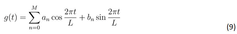
where L represents the duration of the seasonal pattern and 2M +1 denotes the count of parameters involved.

The majority of stochastic differential equations do not have analytical solutions. In this study, the Euler-Maruyama method was employed for discretization to obtain an approximation for a stochastic differential equation.

Definition 6: The Euler-Muryama method given by Y_n+1=Y_n +_a(Y_n,τ_n)Δt+b(Y_n,τ_n)ΔW_n, where ΔW_n=W_τn+1−Wτn and recursively defined Y_n for 0 ≤ n ≤ N-1

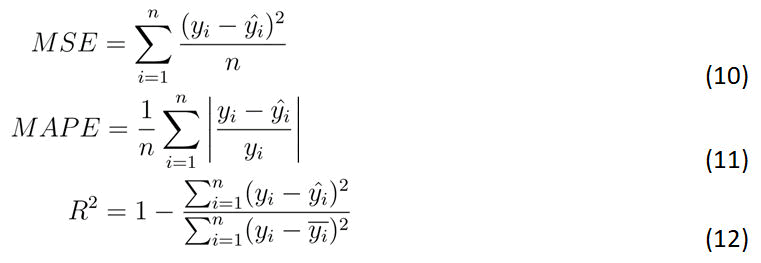
In the context of this analysis, where approximations are necessary due to the inherent complexity of most stochastic differential equations, three key metrics to assess the accuracy and precision of our models were employed. The Mean Square Error (MSE) was used to quantify the extent of both overestimation and underestimation between predicted values and raw data. Meanwhile, the Mean Absolute Percentage Error (MAPE) was used to gauge the reliability of the models in terms of prediction accuracy. Lastly, the coefficient of determination (R²), was used to evaluate the models’ effectiveness in describing variations within the dataset. These measures collectively provided a comprehensive evaluation of the approximations’ performance, which helped to address the challenges presented by stochastic differential equations.

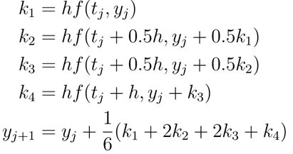
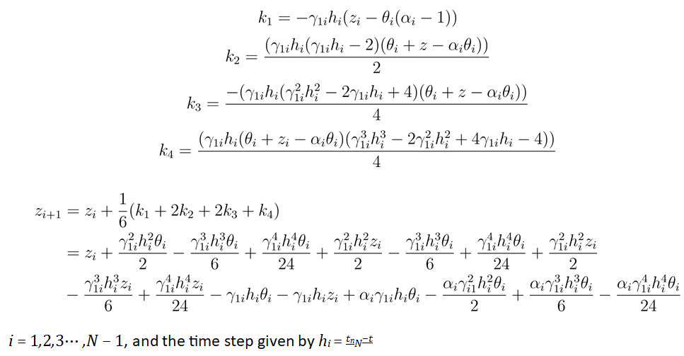
Definition 7: To estimate auto-correlation parameters, both Runge-Kutta and optimization methods were employed.

Definition 8: The form of the fourth-order Runge-Kutta method is as follows:

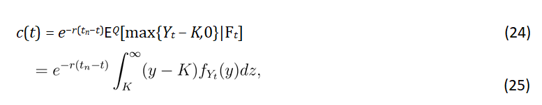
The pricing approach employed the method of expected payoff, as defined in the following description.

Definition 9: The price of the call option, determined by discounting the expected payoff using the available temperature data,is expressed as follows:

Temperature model derivation

The general expression for an Ito stochastic differential equation is provided as follows:

dY_t=μ(Y_t,t)dt+σ(Y_t,t)dW_t            (14 )

μ(Y_t,t) denotes the drift coefficient, σ(Y_t,t) is the diffusion coefficient and W_t is the standard Brownian motion also called the stochastic process {W(t),t ≥ 0} in which P(W(0)=0)=1, E(W(t))=0, Var(W(t))=t, W(t) ∼ N(0,t) and {W(t)-W(s),0<s<t} is independent process. It is the noise only that is normally distributed and not the temperature. This assumption is realistic.

Utilising the synthesis method outlined in Bykhovsky [13] and Kanellopoulos et al. [14], for deriving diffusion equations, we stem the stochastic differential equation governing daily temperature. During this derivation, we make two fundamental assumptions. Firstly, we presume that temperature values exhibit autocorrelation. Secondly, we assume that the normalized covariance function is expressed as

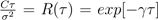
and we define the auto-correlation interval as,

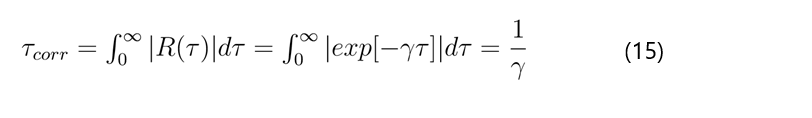
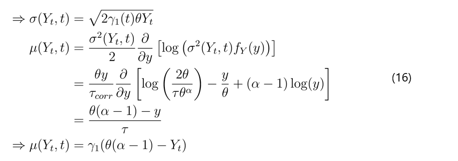
Following the derivation of the stochastic equation presented earlier, we have determined the expressions for drift and the diffusion coefficient as 15 and 16 respectively. Now, by substituting these in 14 we obtain the result as below

dY_t=γ₁(t)(θ(α-1)-Y_t)d_t+p₂γ₁(t)θY_tdW(1)(t)                 (17)

This differs slightly from the Ornstein-Uhlenbeck differential equation in that the diffusion coefficient in 30 is contingent upon the random variable Y_t.

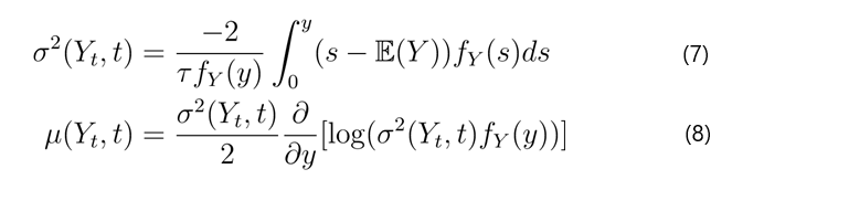
Analysis of the temperature model parameters

Lemma 4: The expected value of (Y) is given by the following differential equation

dz=γ(θ(α-1)-z)dt, where z=E(Y_t)                   (18)

Proof

We apply Ito isometry in equation 30

dE(Y_t)=γ(θ(α-1)-E(Y_t))d_t dz=γ(θ(α-1)-z)d_t

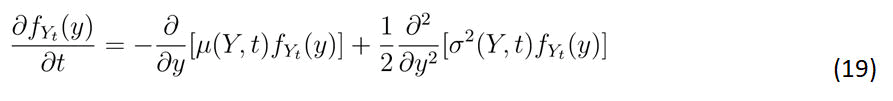
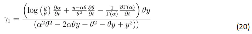
Lemma 5: Suppose that the model in equation 30 satisfies the following FPE.

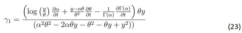
Then γ1 is given by the following equation

Proof

We assume that θ(t) and α(t) are {F_t}−measurable

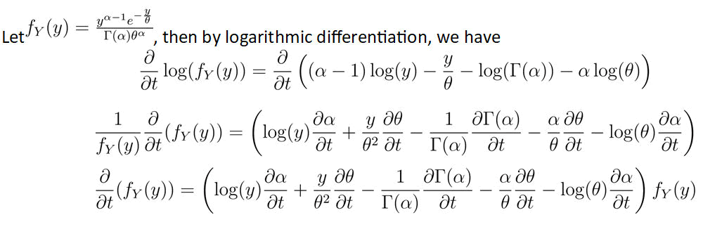
Applying laws of logarithms and simplifying fraction, we get

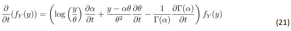
The second operator in the FPE can be expressed as follows

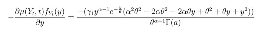
Applying the third operator of the FPE to the stochastic differential equation gives

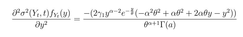
Therefore, the right hand side of the FPE can be expressed as follows

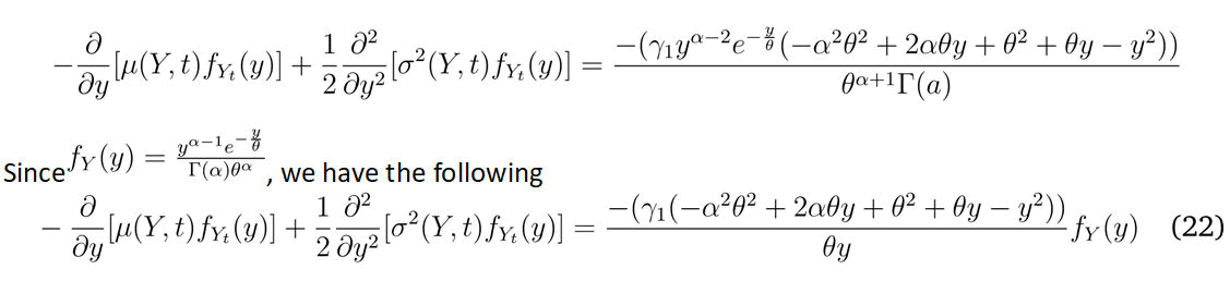
Putting the results in Equation 1(2) and (22) in the FPE an d then solving for γ₁ gives

Numerical estimation of trigger value

A trigger value refers to a specific threshold or level that, when crossed or reached, initiates a specific action or event in a financial instrument or contract. It serves as a condition or criterion that determines when certain provisions or features associated with the instrument come into effect. It varies depending on the context and the specific financial instrument or contract involved. It could be a predefined price level, a specified time period or value of a particular variable, a particular event occurrence or a combination of factors. For example, in options contracts, a trigger value may represent the strike price at which the option is exercised or the barrier level at which a knock-out or knock-in feature is activated.

In order to apply the Runge-Kutta method in equation 18 we let f(t_i,z_i)=γ₁(θ(α-1)-z_i) then,

Forecasting temperature: The parameters α and θ governing scale and shape respectively in the Stochastic differential equation 30, estimated through a combination of Fourier series as outlined in definition 9 and optimization. Subsequently, the Euler-Muryama method as defined in definition 6 and supported by Mao [15], was employed to estimate temperature values. MSE given by equation 10 was used to account for discrepancies between raw and predicted values Willmott and Matsuura, MAPE given by equation 11 was used to assess model reliability, in accordance with Khair et al., and equation 12 was used to gauge the model’s suitability for the given dataset, aligning with the methods presented by Allison et al. Ultimately, pricing was determined by discounting the expected payoff, as specified in equation 13 based on available temperature data at any given time t, ensuring that our model incorporates real-time information.

Pricing temperature derivatives: Taking into account the fact that Y_t follows a gamma distribution, thus, the call option’s price at t ≤ t₁ is given by:

where K=Z_t

Here, Z_t represents the mathematical expectation, which serves as the solution to Ordinary Differential Equation 23, We designate K as the agreed-upon critical or trigger value, which we take to be the predicted average of Z_t and F_t signifies temperature information at time t also known as the filtration. Upon evaluating the integral in Equation 3 the outcome is as follows:

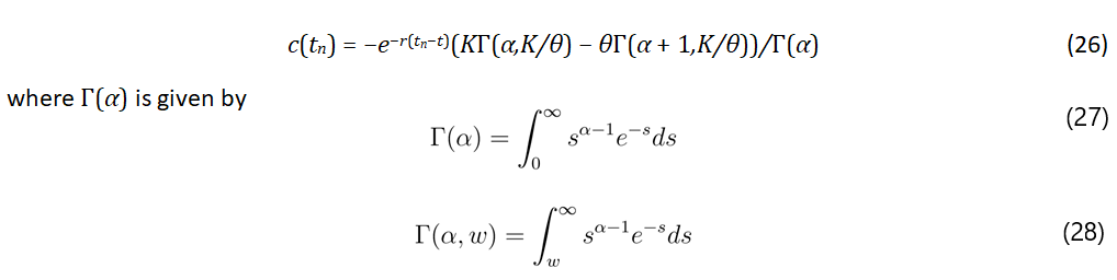
This is referred to as the upper incomplete gamma function, with r denoting the risk-free interest rate, while t and t_n represent the initial and final times of the agreed contract, respectively.

Results and Discussions

This section provides results on modeled temperature, how gamma distribution fits into data collected. It also indicates parameter estimates both alpha and theta as in scale and shape respectively. A sample contract has been demonstrated with an African Risk Company (ARC) and Malawi government. Finally, the paper has also demonstrated the relationship between the call option and trigger value.

Estimating a gamma distribution for temperature data

Temperature (Y) in the area conforms to a gamma distribution. The conventional method typically involves assuming that temperature adheres to the probability distribution described by the Ornstein-Uhlenbeck stochastic process which posits that the residuals, when the trend reverts to the mean, follow a Gaussian probability distribution. However, the research done by Gyamerah et al., suggests that there is a non-negligible probability that temperature residuals may not adhere to a normal distribution.

In previous research, a normal probability distribution was found to be a good fit primarily for maximum temperatures. Haddad demonstrate that the gamma distribution is more appropriate when considering daily temperature data, which incorporates both the maximum and minimum temperatures recorded on a given day. The probability density function of the gamma distribution is described by the function (1). The mean of Y, second moment and variance are given by results in Lemma 2. Similarly, the method of moment estimators of the parameters are given in definition 2.

In this scenario, we estimate E(Y) by the sample mean and Var(Y) by sample variance. To illustrate, temperature data obtained from the Chitedze research station in Malawi, spanning the years from 1981 to 2021 (as available during the writing of this paper) was used. The resulting statistics were as follows.

This study incorporated temperature data collected concurrently with rainfall data. Specifically, all temperature values on days with zero rainfall were excluded from the dataset. Subsequently, the collected data was fitted to a gamma distribution, as illustrated in Figures 1a and 1b where it is evident from Figure 1b that temperature values closely align with the best-fit line, indicating a strong adherence to the gamma distribution [16]. It’s worth noting that the histogram slightly resembles a normal curve due to the presence of a large scale parameter, as detailed in Table 1.

Table 1: Parameter estimates.

Figure 1: Exploring probability distribution of temperature.

To evaluate the goodness of fit of the model, a Chi-square test was employed, as detailed by Balakrishnan et al. utilizing the parameter estimates computed, the chi-square test is defined as follows:

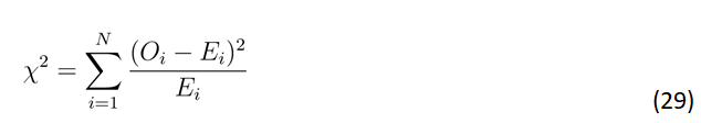
The outcomes indicated that temperature conforms to a gamma distribution as a random variable, with a p-value of 0.9261. This took into consideration the fact that temperature was categorized into seasons like ”winter,” ”spring,” ”summer” and ”autumn.” This categorization allows to treat temperature as a categorical variable for the chi-square test.

The temperature model: The derived temperature model is given by

dY_t=γ₁(t) (θ(α-1)-Y_t)dt+p2γ1(t)θY_tdW₍₁)(t) (30)

The properties of this equation are derived in section 3.1. Such properties give conditions that must be satisfied by the autocorrelation interval coefficients γ₁ for the model to satisfy the Fokker-Planck equation. This approach is also found in the work of Dzupire et al. According to Tabandeh et al., Fokker-Planck equation is responsible for describing how uncertainly spreads in dynamic systems that are influenced by random events. The solution to this equation is a Probability Density Function (PDF) that changes over time and is often of large size and scope. In addition, there are certain characteristics of the joint and any marginal solution PDF that need to remain constant over time. Furthermore, meeting the requirements of the Fokker-Planck equation guarantees that the coefficients γ₁ address issues of non-linear and non-stationary behavior within the data set that may have arisen as a result of climate change.

Parameter estimation: The estimate for the mean α(t)θ(t) was derived using a truncated Fourier series in equation 9. The parameters a_n and b_n were determined through the application of the least square method, as described by Yazdi et al. To estimate variance α(t)θ(t)², the mean square error was computed from

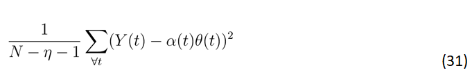
where η is the number of parameters. This value was subsequently multiplied by 1-h_ii, where h_ii are representing influential points in the Fourier series. The obtained results were further modeled using the Fourier series, following a similar approach to that employed by Benth et al. [17], in estimating variance. As a result, we derived estimates for θˆ=α(t)θ(t)²/(α(t)θ(t)) and αˆ=α(t)θ(t)/ (θˆ). The summarized outcomes are presented in Figure 2. Notably, the values obtained in Figures 2a, 2b and 2c correspond to the values listed in Table 1, demonstrating the consistency of this method.

Figure 2: Estimates of α and θ.

Nonetheless, employing maximum likelihood estimation entails assuming that there is independent sampling. Given that this study assumes the presence of autocorrelation within the data and follows a gamma distribution, a different approach has been adopted by using Equation (23). Alternatively, Equation 18 can be solved using the Runge-Kutta method to obtain the sequence Zt. Following this, the parameters were determined by solving the subsequent minimization problem. The results were not different (Table 2).

argminL(γ)=X(Y_i-Z_i)² (32)

Table 2: Estimates of γ.

This provides us with the following estimates for the autocorrelation parameter (γ). In Table 2 shown above, the autocorrelation parameter (γ) exhibits a range spanning from 0.039 to 0.503. With these diverse γ values from Table 2, temperature values were estimated utilizing a stochastic differential equation (30), resulting in the estimated values depicted in Figure 3 below.

Figure 3: Temperature estimation.

Figure 3 depicted above illustrates that the predicted temperature values closely align with the raw data. The predictions and computations encompassed the entire dataset, while the graph specifically displays predictions for the last season, offering a more accessible visual representation. To assess accuracy, we employed the Coefficient of Determination (Rsquared), Mean Absolute Percentage Error (MAPE) and Mean Squared Error (MSE) as defined in Equations 10, 11 and 12, respectively. The coefficient of determination gauges the model’s suitability for the dataset, with values closer to 1 indicating strong alignment between model variations and raw data variations. MSE aids in identifying whether the predictions involve underestimation or overestimation. MAPE quantifies the reliability of the predictions, measuring the percentage of points for which the distance from the mean falls within the MAPE range, as elucidated by Chicco et al. [18].

With an R-squared value of 91%, it can be inferred that the model can explain approximately 91% of the variations in the data, indicating its suitability for the dataset. The MSE value of 0.1429 suggests that the model’s tendency for underestimation or overestimation has been mitigated to within 0.1429 units of the actual data. Furthermore, it’s worth noting that approximately 58% of the data points within the model fall within a MAPE of 1.36% as shown in Table 3, signifying a high level of reliability in the predictions. The performance of this model is comparable to that of Schiller et al. and Benth et al., who used fractional integration together with Bsplines to derive temperature model. Since the reliability is much better than their model, then this model is less expensive than their model.

Table 3: Accuracy and reliability.

Pricing derivatives: The following table shows a sample contract between the African Risk Capacity (ARC) and the Malawi government.

The payout of the contract would be used to support vulnerable communities affected by the temperature variations. In exchange for this coverage, the Malawi government would pay a premium to the ARC, which would be determined based on the level of coverage and the likelihood of the predetermined conditions being met [19,20]. The contract would help the Malawi government to manage the financial risk associated with temperature variations and ensure that vulnerable communities are supported in times of need.

Now suppose we have α=10.15, θ=0.721, then the price of call option per farmer in Table 4 is K9361.

Table 4: Sample contract between (ARC) and government.

Based on the graph in Figure 4 above, it is evident that as the trigger value increases, the premium decreases.

Figure 4: Relationship between call option and trigger value.

This observation suggests that in financial derivatives, an event is less likely to occur when the average trigger value is higher, resulting in lower premiums.

These results obtained using the model (26) are indicating a similarity with the work of Turvey who derives feasible regions of temperature process space in which a farmer is more likely to be paid by a buyer like ARC. This explains why Johnson suggests that those signing the contract with the ARC on behalf of the government should have sound knowledge about the weather derivatives which are temperature dependent. This model is different from that of Karydas and Xepapadeas in that it is independent of initial temperature and volatility. It is also reflecting well as suggested by Cramer et al., in his study using Machine learning. However, the information about the volatility is contained in the parameters α(t) and θ(t). Therefore, this model can be more flexible for pricing temperature derivatives.

Conclusion

The objective of this research was to construct a model for estimating call option prices with temperature as the underlying factor. To accomplish this, several steps were undertaken: a Stochastic Differential Equation (SDE) was developed, temperature was modeled and predicted using this SDE, a pricing model was formulated, and ultimately, call option prices were estimated.

A stochastic differential equation was formulated using the synthesis method, with the assumption that temperature exhibited autocorrelation. This equation demonstrated strong predictive accuracy for weather values.

The pricing model does not directly rely on the underlying temperature as a solution to the Stochastic Differential Equation (SDE). Instead, it explicitly hinges on the gamma parameters and the trigger value. As the trigger value increases, the prices generally exhibit a decreasing trend.

The model is much dependent on the gamma parameters and hence it may be used using intermediate and pre-processed data to price temperature derivatives. Hence, we recommend authors as well as traders of weather derivatives to consider using this model for estimating fair prices of derivatives.

In an extension beyond the scope of this paper, it is possible to consider combinations of any two of the following weather conditions: temperature, wind speed and rainfall, as the underlying factors for pricing call options.

Acknowledgments

I express my profound gratitude to the Almighty for the gift of life. Additionally, I extend my heartfelt appreciation to Dr. Dzupire for his consistent and invaluable support as my supervisor throughout this journey.

References

1. Gyamerah SA, Ngare P, Ikpe D. Regime-switching temperature dynamics model for weather derivatives. Int J Stochastic Anal. 2018;2018(1):8534131.

   [Crossref] [Google Scholar]

2. Andrews L, Shivamoggi B. The gamma distribution as a model for temperature dissipation in intermittent turbulence. Phys Fluids A: Fluid Dyn. 1990;2(1):105–110.

   [Crossref] [Google Scholar]

3. Moriarty M, Murray A, Berx B, Christie A, Munro L, Wallace I. Modelling temperature and fish biomass data to predict annual Scottish farmed salmon, salmo salar l., losses: Development of an early warning tool. Prev Vet Med. 2020;178:104985.

   [Crossref] [Google Scholar] [PubMed]

4. Haddad K. Selection of the best fit probability distributions for temperature data and the use of l-moment ratio diagram method: A case study for NSW in australia. Theor Appl Climatol. 2021;143(3):1261–1284.

   [Crossref] [Google Scholar]

5. He L, Wang Y, Wei Y, Wang M, Hu X, Shi Q. An adaptive central difference kalman filter approach for state of charge estimation by fractional order model of lithium-ion battery. Energy. 2022;244:122627.

   [Crossref] [Google Scholar]

6. Cramer S, Kampouridis M, Freitas AA, Alexandridis AK. An extensive evaluation of seven machine learning methods for rainfall prediction in weather derivatives. Expert Syst Appl. 2017;85:169–181.

   [Crossref] [Google Scholar]

7. Geman H, Yor M. Pricing and hedging double-barrier options: A probabilistic approach. Math Finan. 1996;6(4):365–378.

   [Crossref] [Google Scholar]

8. Hess M. Pricing temperature derivatives under weather forecasts. Int J Theor Applied Fin. 2018;21(05):1850031.

   [Crossref] [Google Scholar]

9. Ahˇcan A. Statistical analysis of model risk concerning temperature residuals and its impact on pricing weather derivatives. Insurance: Mathemat Econom. 2012;50(1):131-138.

   [Crossref] [Google Scholar]

10. Liu X, Shi L, Qian H, Sun S, Wu P, Zhao X, et al. New problems of food security in Northwest China: A sustainability perspective. Land Degrad Develop. 2020;31(8):975-989.

    [Crossref] [Google Scholar]

11. Alaton P, Djehiche B, Stillberger D. On modelling and pricing weather derivatives. Appl Math Fin. 2002;9(1):1–20.

    [Crossref] [Google Scholar]

12. Berhane T, Shibabaw N, Awgichew G, Kebede T. Option pricing of weather derivatives based on a stochastic daily rainfall model with analogue year component. Heliyon. 2020;6(1):e03212.

    [Crossref] [Google Scholar] [PubMed]

13. Bykhovsky D. Simple generation of gamma, gamma–gamma, and k distributions with exponential autocorrelation function. J Lightwave Technol. 2016;34(9):2106-2110.

    [Crossref] [Google Scholar]

14. Kanellopoulos SA, Fikioris G, Panagopoulos AD, Kanellopoulos JD. A modified synthesis procedure for first order stochastic differential equations for the simulation of baseband random processes. Signal Process. 2007;87(12):3063–3074.

    [Crossref] [Google Scholar]

15. Mao X. Convergence rates of the truncated Euler–Maruyama method for stochastic differential equations. J Comput Appl Math. 2016;296:362–375.

    [Crossref] [Google Scholar]

16. Chidzalo P, Abonongo J, Naryongo R. Enhancing reliability and accuracy in stochastic growth modeling: Method of three selected points approach. Comput J Math Stat Sci. 2023;2(2):291-302.

    [Crossref] [Google Scholar]

17. Benth FE, Šaltytė Benth JŪ, Koekebakker S. Putting a price on temperature. Scandinavian J Stat. 2007;34(4):746–767.

    [Crossref] [Google Scholar]

18. Chicco D, Warrens MJ, Jurman G. The coefficient of determination r-squared is more informative than smape, mae, mape, mse and rmse in regression analysis evaluation. PeerJ Comput Sci. 2021;7:e623.

    [Crossref] [Google Scholar] [PubMed]

19. Guiteras RP, Jack BK. Productivity in piece-rate labor markets: Evidence from rural malawi. J Dev Econ. 2018;131:42–61.

    [Crossref] [Google Scholar]

20. Johnson L. Rescaling index insurance for climate and development in Africa. Econ Soc. 2021;50(2):248–274.

    [Crossref] [Google Scholar]