Journal of Aeronautics & Aerospace Engineering
Open Access
ISSN: 2168-9792
ISSN: 2168-9792
Research Article - (2017) Volume 6, Issue 3
This paper identifies feasible fight paths for Small Unmanned Aircraft Systems in a highly constrained environment. Optimal control software has long been used for vehicle path planning and has proven most successful when an adequate initial guess is presented to an optimal control solver. Leveraging computer animation techniques, a large search space is discretized into a set of simplexes where a Dubins path solution is generated and contained in a polygonal search corridor free of path constraints. Direct optimal control methods are then used to determine the optimal flight path through the newly defined search corridor. Two scenarios are evaluated. The first is limited to heading rate control only, requiring the air vehicle to maintain constant speed. The second allows for velocity control which permits slower speeds, reducing the vehicles minimum turn radius and increasing the search domain. Results illustrate the benefits gained when including speed control to path planning algorithms by comparing trajectory and convergence times, resulting in a reliable, hybrid solution method to the SUAS constrained optimal control problem.
<Keywords: Optimal control; Optimization; Unmanned systems; Direct orthogonal collocation; Path planning; Triangulated mesh
The DoD has continued to recognize Small Unmanned Aircraft Systems (SUAS) as critical assets and the demand on their capabilities continues to grow. They are ideally suited for the dangerous or repetitive missions that otherwise require human involvement [1]. Incorporating SUAS into the battlefield will streamline systems, sensors, and analytical tasks while significantly reducing the risk to human life [2]. Across the DoD and civilian industry, the demand for unmanned capabilities has become paramount. Specifically, Manned Unmanned Teaming (MUM-T) is one role SUAS perform that augment and enhance human capabilities with a desired goal to ensure operations in complex and contested environments [3]. Manned aircraft flying through terrain and over urban canyons can experience ground threats that significantly reduce their ability to accomplish the mission. By teaming with SUAS, the manned aircraft can maintain a safe distance from the threat environment while relying on SUAS to augment the mission through system sensors. This scenario becomes ideal if the SUAS can autonomously navigate through a constrained environment from one area of interest to the next without the requirement for human interface.
Optimal control techniques are evaluated herein to determine feasible flight paths for autonomous SUAS through a highly constrained environment. Three common challenges are addressed herein that become problematic when using optimal control software. First, convergence to a solution is not always guaranteed. Second, the computation time required to achieve a solution can vary greatly. Third, constraint modeling and implementation can significantly affect the computation speed and convergence of the problem. Each of these issues can be attributed to the problem formulation, constraint implementation, and the initial guess provided to the NLP solver. Further, system parameters must be bounded appropriately to ensure the space is adequately searched, increasing the number of parameters the user is required to input.
To overcome these issues, insight will be taken from developments in the field of computer animation where Constrained Delaunay Triangulation (CDT) techniques are used to eliminate constraints from the search field and input parameters are generalized through a transformation to barycentric coordinates in a multi-phased approach. Computer animation path planning algorithms have become computationally efficient and perform effectively in moving autonomous agents through simulated environments. However, these algorithms are often restricted to the two-dimensional plane with limited control on the agent. Combining these path trajectories with the increased capabilities of optimal control software allows for efficient, feasible, multi-control solution for autonomous SUAS flight.
Numerical solutions to optimal control problems are often solved with indirect or direct methods. Indirect methods use the calculus of variation to form the Hamiltonian, resulting in a two-point boundary value problem. The optimal solution is determined by solving the first-order optimality conditions while minimizing the Hamiltonian with respect to the control. With this method, a good approximation is required for the states, co-states, control and time. However, the optimality conditions can often be difficult to formulate and determining a realistic estimate of the co-states is not intuitive.
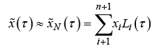
Alternatively, direct methods transcribe the infinite-dimensional optimal control problem into a finite-dimensional optimal control problem with algebraic constraints, also known as a Nonlinear Programming (NLP) problem [4]. Solutions are acquired using orthogonal collocation methods, polynomial approximation of the state, and numerical integration through Gaussian quadrature. The state, X, is approximated at a set of collocation points described as
 (1)
(1)
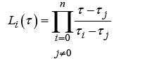
where xi represents the weight function, Li(τ) is the Lagrange polynomial basis
 (2)
(2)
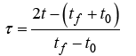
and τ represents an affine transformation of the time t on the interval (-1, 1)by
 (3)
(3)
This method is termed global as each collocation point is solved simultaneously rather than other fixed interval methods such as a 3 or 5 point formula method [5].
One disadvantage of the direct method results from the discretization of the optimal control problem producing several minima, leading to a solution that may be far from the optimal. To minimize this affect, an accurate prediction of the solution, control, and time are required to assure feasible results as there is no guarantee of convergence to a global minimum with direct methods. Many algorithms have been proposed previously to acquire an initial guess to the solution, including Dubins path algorithms [6] and heuristics [7,8] with computation time and accuracy being the limiting factor for complete hybrid solutions. The research herein examines the effectiveness of using computationally efficient path planning algorithms from the field of computer animation to seed the NLP used in the optimal control software for SUAS path trajectories in constrained environments.
To properly formulate the SUAS path planning optimal control problem, all state and control variables must be defined and properly bounded and an initial guess to the path solution, control, and time must be formulated. Often, determining realistic bounds on the states, control, and time can be challenging. Bounds that are set too loose can result in high computation times while setting bounds too tightly can limit the solution search space. Further, solution accuracy and computation times are greatly dependent on the quality of the initial guess used to seed the NLP. To minimize the impacts of these issues, the optimal control problem is formulated in a phased approach. The search space is discretized into a CDT and translated into barycentric coordinates, providing standardized bounds on the system states. Path planning algorithms designed for computer animation are used to achieve feasible path solutions and are formulated to provide a quality initial guess for the states, control, and time in the optimal control problem.
An extensive review of path planning through environments with clearances is given by Kallmann [9]. Algorithms to determine shortest paths while providing a minimum clearance to all constraints are provided by Kallmann [10]. These algorithms focus on computational efficiency while also providing a framework for dynamic addition and removal of constraints. These algorithms have been implemented in the 2010 version of the Tripath toolkit1. An overview of the relevant algorithms from the Tripath toolkit is given below; a more extensive review of the algorithm can be found by Kallmann [9,11].
First, let G consist of a planer straight-line graph with S defining a set of n segments that form all the constrained edges in the domain. A CDT, T, is then formed such that all segments of S are also segments of T and the constrained Delaunay criterion defined below are upheld.
For each unconstrained edge e of T, there exists a circle C such that
1. The endpoints of edge e are on the boundary of C
2. If any vertex v of G is in the interior of C then it cannot be “seen” from at least one of the endpoints of e [12].
Figure 1 illustrates the CDT for a single polygonal constraint.

Figure 1: CDT of polygonal constraint.
With this technique, constraints can effectively be forced in the discretization of the space. In computer animation, these constraints represent walls, furniture, and other common obstacles an autonomous agent must avoid when traversing through a space. To account for the width of the autonomous agent, a test is performed to assure a disk of radius r can traverse through any given region without crossing a constrained edge. This allows for an efficient computation of paths of arbitrary clearance. To assure the accuracy of the feasible paths, a local clearance test is performed to verify a path solution with minimum radius of 2r. In the event a path corridor is restricted, a refinement of the mesh is attempted by redistributing the triangulation or adding a vertex point to a straight line segment of the set S. The final triangulated mesh is then termed a “Local Clearance Triangulation (LCT)”.
A path through the LCT is defined as a “free” path if it traverses from an initial point p to a final point q without crossing a constrained edge. A free path will cross several unconstrained edges resulting in a “channel” of connected simplexes formed of all traversed triangles. A path solution through this channel is determined with a “funnel” algorithm developed by Lee and Preparata, and Chazelle [13,14] as cited by Hershberger [15]. The funnel algorithm has been demonstrated under multiple applications, including path finding for autonomous agents [16], querying visible points in large data sets to define shortest paths [17], shortest paths for tethered robots [18], and robots in extreme terrain [19].
Given a corridor defined by a series of triangles, the funnel algorithm determines the shortest path from an initial point p to a final point q, subject to a defined clearance from each simplex edge. The apex of the first triangle is defined as a, with the remaining two vertex points on the shared triangle edge defined as u and v. The remaining vertex of the second triangle is defined as w. If the straight line path from a to w is feasible, that path is stored as shown in Figure 2A. Maintaining a as the apex, the straight line path from a to the following triangle vertex point, w’ is evaluated for feasibility and stored if accepted, as shown in Figure 2B. This process continues until a straight line solution fails upon which the vertex providing the shortest distance to the next point in the path is chosen as the new apex, a’ and the algorithm continues as shown in Figure 2C. A detailed description of the funnel algorithm can be found in Hershberger’s work [15]. Finally, in order to account for local clearances around obstacles, a circular constraint of radius r is imposed on each vertex point as illustrated in Figure 2D [11].

Figure 2: Tripath path development.
The Tripath toolkit utilizes an A* search algorithm to provide a locally optimal search, defining a Dubins path solution contained in a series of triangles. It is capable of achieving path solutions on the order of milliseconds for environments with 60K+ segments [9]. This path solution can be translated to the SUAS problem by setting the radial clearance distance of each vertex equal to the turning radius of the SUAS, therefore providing a feasible path to seed the NLP. Although there is no guarantee that the defined search corridor will contain a global solution, it will guarantee a feasible flight path that is free of constraints when exogenous inputs are excluded. Currently, the Tripath algorithm results only produce a path solution without influence of control parameters or rate limits. Although the algorithm is computationally efficient, additional work is required to produce SUAS flight trajectories while fully exploiting vehicle control parameters throughout the problem domain.
With a feasible path solution acquired to seed the NLP, the parameter bounds on the states, control, and time of the optimal control problem can be simplified with a translation from the Cartesian coordinate frame to the barycentric coordinate frame. Often, when dealing with simplex shapes, the barycentric coordinate frame is preferred in which the location of a point within a simplex shape is defined as a weighted measure to each of the vertices, also referred to as areal coordinates when restricted to the two-dimensional simplex [20].
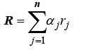
Defining the coordinate system in  ,let r1, r2, and r3 be vertices of a simplex G. Any point, R, inside simplex G can be represented in terms of the vertices of G and the barycentric weights, used as a basis as follows [21-23]:
 (4)
(4)
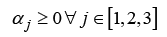
where αrepresents a set of real coefficients, defining the barycentric weights whose sum equals unity and r defines the vertex points in Cartesian coordinates. Requiring the weights to be positive semidefinite ensures the point is maintained inside simplex Q,
 (5)
(5)
The simplex parameters illustrating Cartesian coordinates in R and barycentric coordinates in A is shown below in Figure 3.

Figure 3: Barycentric coordinate frame.
For the two-dimensional triangular relationship, transformation from a barycentric coordinate frame to a Cartesian coordinate form can be accomplished through the linear transformation
 (6)
(6)
where R∈defines the point location inside the simplex in Cartesian coordinates, Q∈ defines the vertex matrix of simplex G comprised of vertex points
  , and
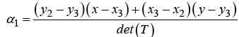
, and defines the barycentric weight matrix. Expanding Equation 3 and solving for the first two barycentric coordinates yields
 (7)
(7)
where T is a 2x2 matrix comprised of the vertex points of simplex Q,
 (8)
(8)
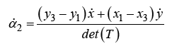
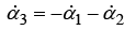
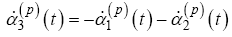
and third barycentric weight, α3, is expressed in terms of the first two calculated weights to sum to unity.
Expanding Equation 4 yields the barycentric weights in terms of both the interior point location and the vertex points of the simplex.
 (9)
(9)
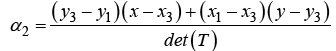 (10)
(10)
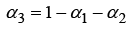 (11)
(11)
Differentiating the weights with respect to the x and y position allows for the propagation of dynamic state equations through an individual simplex.
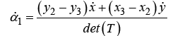 (12)
(12)
 (13)
(13)
 (14)
(14)
Evaluating the determinant of matrix T, singularities will become problematic only if the vertex points of the simplex become collinear. By defining the discretization of the search space to hold the properties of a CDT, singularities in the dynamics will be avoided.
The optimal control problem is formulated in the General Purpose Optimal Control Software (GPOPS-II) and implemented in MATLAB. GPOPS-II is a computation tool for solving multiple-phase optimal control problems using variable-order Gaussian quadrature collocation methods with an adaptive mesh refinement [24]. The user is required to input parameter bounds on the initial, intermediate, and final states, as well as the time vector, control, and any additional path constraints presented in the scenario.
By discretizing the problem’s search space with a CDT, the path through each individual simplex can be represented in GPOPS-II as a single phase, each with a specified set of dynamics, constraints, and bounds. The solution acquired from the Tripath toolkit provides both the initial guess of the path solution as well as the simplex structure to effectively formulate the optimal control problem in GPOPS-II.
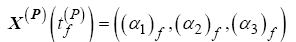
The output of the Tripath algorithm yields three text files containing the path solution, the CDT, and the defined search corridor. The discretized path solution contains the endpoints of each straight line path and equally spaced points of constant radius on each turn. To properly formulate the initial guess, the solution, CDT, and the search corridor are translated to barycentric coordinates and the path is interpolated and subdivided into each simplex equating to the optimal control phases. As the path trajectory traverses across a simplex edge, the vertex points from the current phase to the next must transition such that the barycentric weights appropriately reflect the active vertex points. This process is illustrated below in Figure 4.

Figure 4: Simplex phased solution.
Here it can be seen that as the path solution approaches a simplex edge, the state corresponding to the opposite vertex has no contribution to the location of the point and therefore accepts a zero value. Care must be taken to assure the state vector accurately represents the corresponding weight values as the path transitions across the simplex boundaries.
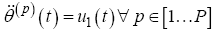
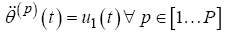
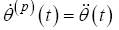
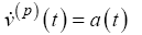
The aircraft dynamics for this problem are derived in the twodimensional plane, representing constant altitude flight. They are formulated with a five state model describing the SUAS position in the x(t ), y (t ) directions, the heading angle, , the heading rate, , and the velocity u(t ) .The control, u(t ), is implemented on the derivative of both the heading rate, , and the velocity,
 (15)
(15)
 (16)
(16)
 (17)
(17)
 (18)
(18)
 (19)
(19)
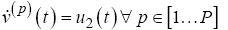
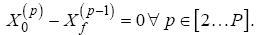
Here, v represents the velocity, p represents the current phase, and P defines the total number of phases in the solution, consistent with the number of simplexes in the defined search corridor.
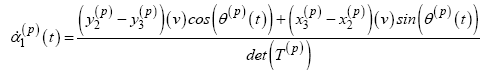
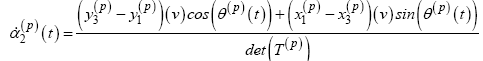
In order to fully transform the SUAS state vector into the barycentric coordinate system, Equations 15-16 are substituted into Equations 12- 13 to form the final set of dynamic equations, ∀ p∈[1…P] .
 (20)
(20)
 (21)
(21)
 (22)
(22)
 (23)
(23)
 (24)
(24)
 (25)
(25)
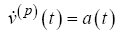
The control is implemented on the derivative of the velocity and heading rate,
 (26)
(26)
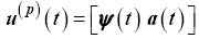
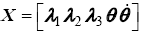
The state vector is defined with six states, represented as
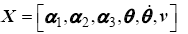 (27)
(27)
Subject to these dynamic constraints, the objective for each scenario herein is to minimize the cost functional
 (28)
(28)
 (29)
(29)
given the initial and final boundary constraints describe as
 (30)
(30)
 (31)
(31)
where the heading, heading rate, and velocity are free variables in the initial and final state. Further, inequality constraints are implemented to maintain the search space within each simplex and provide bounds to the state, control and time defined as
 (32)
(32)
 (33)
(33)
 (34)
(34)
 (35)
(35)
 (36)
(36)
 (37)
(37)
 (38)
(38)
 (39)
(39)
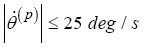
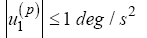
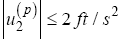
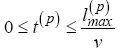
where lmax describes the longest edge of the current simplex. The bound on the fourth and fifth state were chosen to represent a general group 1 SUAS [1]. The bound on the heading rate control was chosen such that the  vector represented an appropriate set of dynamics to implement in an aircraft control system.
Finally, event constraints are implemented to assure a continuously smooth transition of the state variables as the path traverses through each phase, described as
 (40)
(40)
Two scenarios were evaluated to illustrate the savings in the objective cost when solving for constrained path trajectories with the optimal control software, GPOPS-II. In each scenario presented, all polygon constraints are convex, however the approach can be applied to arbitrary polygons. The first scenario considered an aircraft flying at max speed with control limited to only the change in heading rate. This reduces the previously defined state matrix in Equation 27 to a five state model defined as
 (41)
(41)
while the control, previously defined in Equation 26, is reduced to
 (42)
(42)
The Tripath solution was determined with a maximum radial offset distance defined by the vehicles bank angle limit when flying at max speed. The path results, along with the CDT discretization, were used as inputs to seed the NLP of the optimal control software.
The second scenario is constructed to illustrate the advantages of path planning when allowing for speed control on an air vehicle. Again, the Tripath algorithm is used to determine an initial path solution and CDT discretization. In contrast to the first scenario, the radial off-set distance is now defined using the minimum allowable air speed of the SUAS. This reduces the minimum turn radius and may increase the feasible search space of the problem. The optimal control problem consists of the six state, two control model defined previously.
For both scenarios, the SUAS is required to fly through a predefined area of downtown Chicago, USA, measuring 5600 x 2800 ft. The altitude of the SUAS is restricted to 600 ft AGL and therefore all structures exceeding a height of 550 ft are modeled as path constraints that must be avoided. The initial and final locations of the path are defined as
 (43)
(43)
 (44)
(44)
The final location of the scenario was chosen such that the most direct path would require the SUAS to navigate through narrow building corridors requiring minimum radius turns thus illustrating the search domain of the problem.
The initial guess of the path trajectory supplied to the NLP solver is acquired through the Tripath algorithm as described previously. The initial guess of the heading vector is determined by the angle between consecutive Cartesian coordinates of the Tripath solution. The heading rate and control are calculated with a right point finite differencing method initiated with the heading angle vector. Each of these vectors are rate limited to remain consistent with those used in the optimal control problem as in Equations 36 and 37. The initial guess for the velocity vector is formulated with maximum speed on straight sections of the path and minimum speed on the minimum radius turns while the acceleration vector is initiated with the zero vector. The time vector is approximated through each phase as the running summation of the Euclidean distance between consecutive points divided by the vehicle airspeed.
The constraint map is shown below in Figure 5 with each building exceeding 550 ft described with a red enclosed polygon. Building heights were estimated in order to construct a formidable optimal control problem. The initial and final path locations are shown with green and red asterisks respectively.

Figure 5: Chicago constraint map. Map Data @2017 Google.
The GPOPS-II user settings defined for each scenario are described as shown in Table 1.
| GPOPS-II User Settings | |
|---|---|
| Mesh Method | hp-PattersonRao |
| Mesh Tolerance | 10-2 |
| NLP Solver | SNOPT |
| Method | RPM-differential |
| Derivative Supplier | AdiGator |
| Derivative Level | First |
| NLP Tolerance | 10-3 |
| Min Collocation Points | 4 |
| Max Collocation Points | 10 |
| Mesh Fraction | 0.5*ones(1,2) |
| Mesh Collocation Points | 4*ones(1,2) |
Table 1: GPOPS user defined settings.
The optimal control problem for the first scenario is as described previously with the objective being to fly from the initial point to the final point in the shortest amount of time. Often, with minimum time SUAS problems, the path solution is flown at maximum speed, therefore this problem only allows a single control defined as the change of heading rate of the vehicle.
Scenario #1: Tripath solution
The Tripath algorithm is solved and implemented as the initial guess to the NLP. It is initiated with the polygonal constraints, the initial and final location of the path solution, and a defined off-set distance from each constraint. To assure a feasible flight path solution, the radial off-set distance is determined through the relationship between the vehicles velocity and turn rate as follows,
 (45)
(45)
for R is the minimum turn radius, v is the velocity, and ω is the turn rate. For this scenario, the max velocity was set to 30 ft/s with a turn rate of 25 deg/s yielding a turn radius of 68 ft. The resulting search corridor and path solution are shown in Figure 6.

Figure 6: Max radius Tripath solution. Map Data @2017 Google.“
The Tripath solution is solved in 4.07 milliseconds on a PC resulting with an objective time of 134 seconds. Here the constraint off-set distance is shown on each polygonal vertex with blue circles. Due to the narrow corridors defined between buildings, and the maximum required off-set distance, the only feasible path solution requires the SUAS to fly around the constraints as shown in the black outlined simplex search corridor. The path solution is shown as a Dubins path made of up straight line sections and max radius turns. However, this path is not optimal due to the placement of the circular off-set constraints placed on the vertex of each polygonal constraint. This allows for improvement to be seen in the objective function when solved with an NLP.
Scenario #1: GPOPS-II solution
The path results for the optimal solution through the defined search corridor is shown below in Figure 7.

Figure 7: Sim #1 GPOPS-II Solution. Map Data @2017 Google.
The optimal solution is solved in 2.12 seconds with an objective of 129.9 seconds. The Tripath solution used to seed the NLP solver, SNOPT, is shown with the red dashed line while the discretized optimal solution is shown with the blue asterisks. A small improvement in the objective is seen over the Tripath results but at the cost of computation time.
Figure 8 describes the heading, heading rate, and control respectively. The initial guess formulated from the Tripath results can be seen with the red lines while the optimal solution is shown in blue.

Figure 8: Sim #1 GPOPS-II states and control.
Here, the difference in the two solutions is shown as the Dubins Tripath solution requires max radius turns at each vertex along the path while the optimal control solution can blend the solution through the constrained field.
Although there are benefits to the optimal control solution, justification for using the optimal control software cannot be made at this point given the computation time required to achieve a solution with only minimal improvement to the objective.
The optimal control problem for the second scenario consists of the six state, two control model as described previously in Equations 20-39.
Scenario #2: Tripath solution
The Tripath solution is again initiated with the polygonal constraints, the initial and final location of the path solution, and a defined off-set distance from each constraint. With the velocity now being a state, the SUAS has the ability to reduce speed in order to achieve a smaller turn radius and therefore navigate through narrow city corridors. However, within the constraints of the 2010 Tripath toolkit, the turn radius cannot be varied during a simulation. This limits the Tripath algorithm to solve for a solution using the minimum speed turn radius calculated from Equation 40, yielding a minimum turn radius of 22.9 ft at the SUAS speed of 10 ft/s. The Tripath results are shown below in Figure 9.

Figure 9: Min radius Tripath solution. Map Data @2017 Google.
Similar to the first scenario, the Tripath solution resulted in just 6.1 milliseconds, but at an objective time of 364 seconds which is significantly increased due to the minimum speed restriction. Again the constraint off-set distance is shown with blue circles around each vertex of the search corridor and the path solution is shown with the solid red line. Under minimum speed, the search corridor provides a feasible search space that is a more direct route to the finish location. Although the distance traveled is significantly decreased, the objective time for the Tripath solution is too long to consider this a viable solution in itself.
Scenario #2: GPOPS-II solution
The Tripath solution will again be used as the initial guess to seed the NLP solver SNOPT. Due to the increased objective time of the minimum turn radius Tripath solution, the input vectors are scaled in time to represent a maximum speed solution during straight sections of the path and a minimum speed solution during the constant radius turns.
Implementing the optimal control problem as described previously, but now incorporating control on the SUAS acceleration, the optimal solution through the defined search corridor is shown below in Figure 10.

Figure 10: Sim #2 GPOPS-II solution. Map Data @2017 Google.
The optimal solution is solved in 2.86 seconds with an objective of 120.4 seconds. Here the Tripath solution, post processed for speed control, is shown with the red dashed line while the optimal solution is shown with the blue asterisk. The computation times are similar to those found in the first GPOPS-II simulation, however, by allowing control on the SUAS speed, objective times can be significantly reduced, allowing the vehicle to traverse a more direct path to the target location.
Figure 11 describes the heading, heading rate, heading rate control, velocity, and acceleration control respectively. The initial guess formulated from the Tripath results can be seen with the red lines while the optimal solution is shown in blue.

Figure 11: Sim #2 GPOPS-II states and control.
Similar to the first solution, the Dubins path solution resulting from Tripath can be seen in the top subfigure but here it is acquired with minimum radius turns. By formulating the problem with optimal control software, the turn points in the path can be optimized through the constraints. Further, the 4th subfigure shows the velocity is maintained at max speed for the optimal solution, thus providing a feasible path solution that is direct to the target location and flown at maximum speed. Table 2 below summarizes the simulation results.
| Control | Solution Method | NLP Seed | Objective Time (sec) | Computation Time | |
|---|---|---|---|---|---|
| ψ | Tripath | N/A | 134 | 4.07 ms | |
| ψ | GPOPS-II | Tripath | 129.9 | 2.12 s | |
| a,ψ | Tripath | N/A | 364 | 10.4 ms | |
| a,ψ | GPOPS-II | Tripath | 120.4 | 2.9 s | |
Table 2: Simulation results.
This work demonstrated a solution technique to solve feasible path solutions for SUAS through a highly constrained environment. Leveraging computationally efficient algorithms developed for computer animation, a CDT was performed on the search space and a Dubins path solution was determined through a simplex search corridor, free of all path constraints. The defined search corridor, dependent on the user supplied radius off-set distance set in the Tripath algorithm, defines the domain of the optimal control solutions space. By initiating Tripath with a SUAS maximum speed turn radius, path results are restricted to wide simplex corridors, excluding many routes on the interior of the domain. Although these solutions are flown at maximum speed, the path is often highly sub-optimal. On the contrary, by initiating the Tripath algorithm with the SUAS minimum speed, the defined off-set radius is reduced and path corridors through the interior of the city are included in the solution space. These solutions provide more direct routes to the final location, however, the flight time required to accomplish the path is excessive at minimum speeds.
Optimal control software is utilized to blend the two Tripath results by allowing for control on the SUAS acceleration, enabling the aircraft to optimize the speed profile while determining a path solution through a more direct route on the interior of the city. Using the minimum SUAS turn radius to initiate the Tripath algorithm, a Dubins path solution is acquired and used as the initial guess for the NLP. This result alone is sub-optimal as the Tripath algorithm places the minimum turn radius path constraints on each vertex of the search corridor, defining the Dubins path. The optimal control software is able to improve on the Tripath solution by flying a more direct path while maintaining maximum flight speed, improving the objective function by over 8% on the most direct route.
Speed control in previous path planning algorithms for minimum time objectives, are often not included due to the complexities inherent to the design. This effort has demonstrated the benefit speed control can have in determining efficient flight trajectories in highly constrained domains. Ultimately, by including acceleration control on the SUAS, computational efficiencies and trajectory solutions, provided by the Tripath algorithm, can be exploited with optimal control software to produce accurate and efficient path results in minimum time.
The authors would like to thank the Air Force Research Laboratory, Aerospace Systems Directorate, Power and Controls Division, who sponsored the work and provided the challenging problem concept, background, information, and continual support.