Journal of Geology & Geophysics
Open Access
ISSN: 2381-8719
ISSN: 2381-8719
Research Article - (2016) Volume 5, Issue 5
Seismic waves are used in many fields. It can be applied on determine subsoil structure, and materials. In this work use seismograph for the measurement seismic wave propagation velocity in the real geological (subsoil layers) medium. These investigations are applied in petroleum research institute Egypt. Predication results of subsoil layers thickness and seismic wave’s velocity analysis are obtained. The seismograph recorded receiving sample data from geophones and by “SeisImager” software is extract the final seismogram. The seismograph is dependent on Snell law for wave’s propagation. The obtain result of P and S waves of this work are the same as P and S waves references. P waves are shake ground in the direction they are propagating (longitudinal waves), and S waves are shake perpendicularly or transverse to the direction of propagation.
Keywords: Seismic waves; Seismograph; Usage; Data processing; Layers; Layers samples analysis
The propose work are determine subsoil layers and measure P and S-waves velocity. The propose applied experimental work is implemented in petroleum research institute zone Egypt, the experimental location between latitudes 30-02-42.13N and longitudes 31-20-27.66E as shown in Figure 1. The seismic wave’s propagations are Unique; they are used in many fields. Features of the seismic reflection and refraction waves applicable to many fields [1,2] these fields are subsoil structure, carbonate layer, gas reservoir, and groundwater. Seismic wave generated under the action of the short pulse is a complex wave that consists of the following components as shown in Figure 1. These components are longitudinal compressive P-wave, Transverse S-wave, and Rayleigh-Surface R-wave. Longitudinal P-waves and transverse S-waves are known as the body waves. Body waves are propagating through the medium by means of the hemispherical wave front. The type of the component being considered depends on the source of vibrations. Rayleigh wave which is propagated radially and has the cylinder-like wave front. It is appears simultaneously with the body waves. Displacement of the ground is the vertical direction.
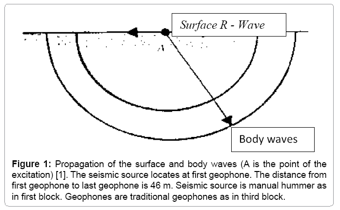
Figure 1
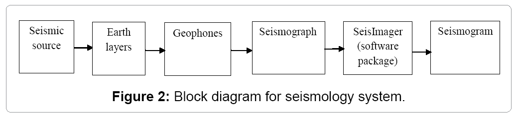
Figure 2: Block diagram for seismology system.
First block is seismic sources
Seismic sources are vibration sources. It generates sound waves. These waves penetrate the earth layer. The seismic sources must be strong vibrator. There are many types of seismic sources. Seismic sources on land and seismic sources on water, but the most often used sources for land surveys are vibrator trucks and for marine surveys are air guns. In this investigation used manual hummer. It is weight 5 Kg. From Newton second law F=max, It is expressed in Newton (N) or Kg m/s2 where m is mass and a is acceleration of mass in x direction. This acceleration from personal thumps the earth layers. For three dimension F=m (ax+ay+az).
Second block is earth layers
All material in subsoil layers make layer. These layers have different thickness. Seismic waves penetrate the subsoil layers has low frequency, high amplitude and high wavelength. The P and S waves equation as following [2,3].

 Where elastic constants are k=bulk modulus, μ=shear modulus and ρ=density of material (subsoil layers). The seismic waves speed (Vp and Vs) changed from layer to another dependent to density and porous of the rock layers, some reading value of Vp and Vs in sandstone and carbonate. Obtain P and S waves by applied these equations.
An applied a force to real object causes some deformation of the object i.e. change of its shape. If the deformation is negligibly small this body considers a rigid body. The rigid body retains a fixed shape under all conditions of applied forces (original shape). If the deformations are not negligible, we have to consider the ability of an object to undergo the deformation i.e. its elasticity, viscosity or plasticity [4]. The refraction or angular deviations that sound rays (seismic pulse) undergoes when passing from one material to another depends upon the ratio of the transmission velocities of the two materials. The fundamental law that describes the refraction of sound rays is Snell’s Law and this together with the phenomenon of critical incidence is the physical foundation of seismic refraction surveys p-waves [5]. Snell’s Law and critical incidence are shown in Figure 3A, velocity V1 underlain by a medium with a higher velocity V2 incidence are shown in Figure 3A.
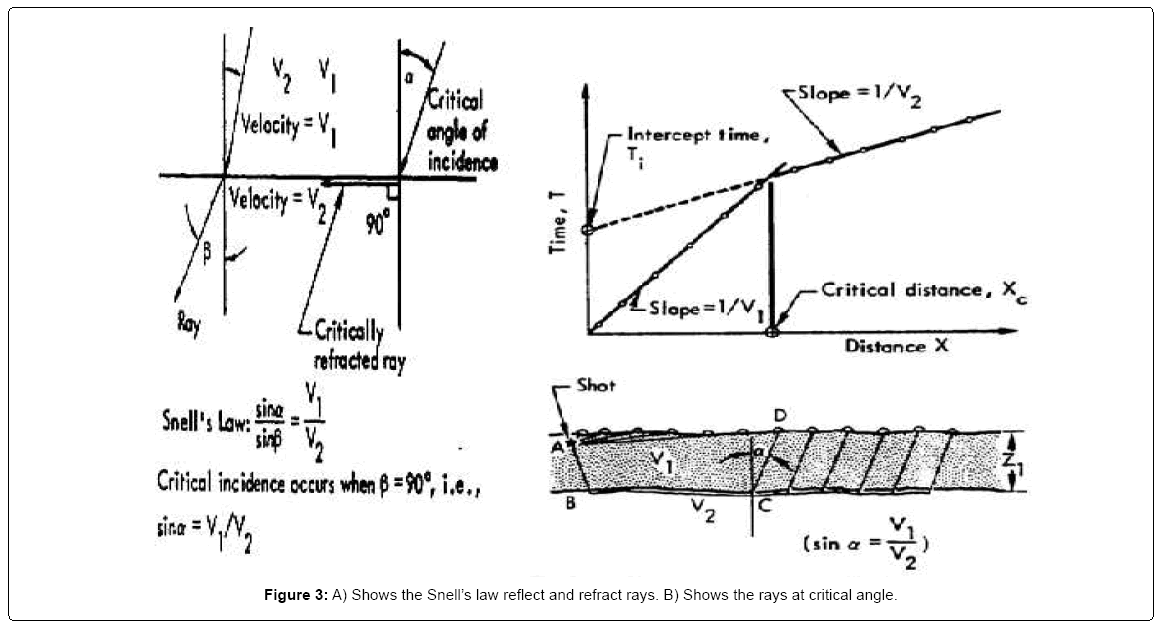
Figure 3: A) Shows the Snell’s law reflect and refract rays. B) Shows the rays at critical angle.
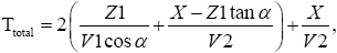
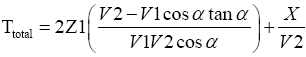
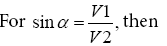
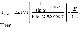
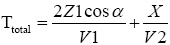
The layers thickness by applied Snell’s [5] as shown in Figure 3,  at β=90 this is critical angle then the rays totally refracted
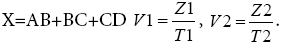
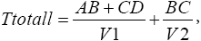
At Boundary between the two layers then the equation become  from Figure 3B Z1 and Z2 are thickness of layers 1 and 2. AB from source to layer 2 then the rays totally refraction from B to C the rays reflection from C to D. AB=CD and
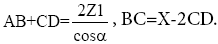
CD=Z1tanα

As shown in Figure 4 multi layers but in our study we applied on two layers.
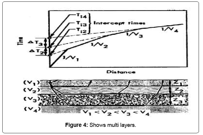
Figure 4: Shows multi layers.
Third block is conventional geophones
Geophones are instrument to sense and measure velocity seismic waves. There are two types of geophone based on application, on land or on water, it is called hydrophone. Most of the geophones are based on the principle of moving coil as shown in figure. The Figure 5 shows geophone structure. It is composed of voice coil suspended inside permanent magnetic. The voice coil is suspended by spring and it is free movement. The voice coil can move up and down inside the magnetic field and produce a voltage Vg. Total spread geophones in this study as shown in Figure 6. Geophones are distributed in horizontal line. Reflected and refraction signals are received by geophones and transmitted from geophone to seismograph by a spread cable. The total geophones distance from first to last geophone (Figure 6) should be 3 to 5 times the depth of interest (depth recommended of seismograph).
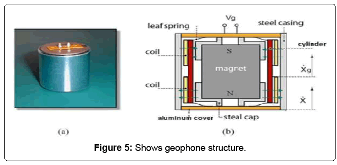
Figure 5: Shows geophone structure.
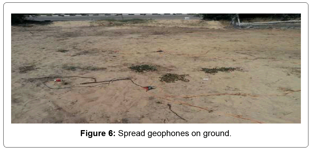
Figure 6: Spread geophones on ground.
In this experiment is 46 m. Seismic source at a minimum there should be two shots located at either began and end of line. It is best practice to also have one center shot (S3) so in our experiment we made three shot (S1, S2 and S3) [5].
Fourth block is seismograph
Seismograph generally consists of sensors (geophones), a low-pass anti-aliasing filter, analog to digital (A/D) converter, and a recorder. Modern digital seismographs are complicated by the extensive electronic circuitry involved [6]. Seismograph used in this experiment as shown in Figure 7.
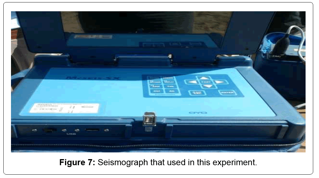
Figure 7: Seismograph that used in this experiment.
Seismograph model
OYO McSeis-SX24, the seismography McSEIS-SX is a portable and it have a 24 channel for a 24 geophones to refraction exploration downhole P-S velocity logging and crosshole seismic for engineering and construction. This is also used as a data acquisition system for multi-channel surface wave analysis. The system is compact, light in weight to transport and do the job with a smaller 12VDC battery anywhere. It’s based on the Windows XP SP2 professional with XGA/ TFT colour display, hard disk drive, USB2.0 ports with higher quality and reliable field performance [7].
The seismic waves transmitted from seismic source impulses subsoil layers, and received by geophones. The impulses transmit from seismic source to subsoil layers from point to another under the influence of an external impulse. Particles of matter in the subsoil layers move from seismic source positions toward each other and collide, and thereby transmit mechanical motion subsoil layers from one point to another. Particles of matter in the subsoil layers begin to vibrate in the direction of seismic wave propagation. The elastic waves propagate and transmit mechanical energy from one point to another as shown in Figure 8. The seismograph represented an oscilloscope in Figure 8. Times elapsed from sending to receiving a seismic wave depend on depths of studied structures and velocities of propagation of seismic waves in medium.
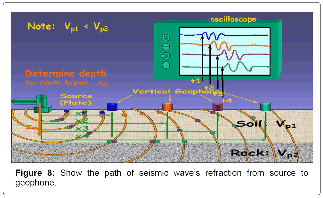
Figure 8: Show the path of seismic wave’s refraction from source to geophone.
The seismograph setting as following below [7]
1. Sample interval: 0.125 to 0.25 mill second (over-sampling is fine) in our experiment is 200 micro second.
2. Data length: 0.25 to 8 k (should be long enough to capture distant arrivals) in our experiment is 4 k.
3. Stacking as needed to increase signal to noise ratio, 5 to 10 times in our experiment is auto (automatic).
4. Delay: -10 ms allows the first break on the near geophones to be more easily viewed in our experiment is zero.
5. Acquisition filters acquisition filters are not recommended because effect is irreversible; should be carefully applied to filter signal you are certain you will never want such as 60 Hz power line noise.
6. Preamp gains highest setting in our experiment are gain 1: set and gain 2: set.
7. Display gains: Fixed gain (same gain over time for a given trace, but variable from trace to trace; traces far from the source will need a higher gain setting than those that are near).
The seismograph settings above are set and now the seismograph is already to receive. To initiate mechanical force explosives hammer. Successful application of seismic methods is based on the fact that subsoil layers have different elastic properties and density that directly depend on their lithological composition [8,9]. Analysis of thus changed properties of seismic waves therefore allows determining the tectonic structure of the subsoil layers, lithological composition of subsoil layers strata, and in favorable circumstances also directly locating reservoirs of oil and gas.
Analyze waveform file of the first shot as shown in Figure 9. Quality is little prefirst break noise, the first breaks are obvious. When there is one refractions break in slope indicates there are another layers. The crossover distance is Break in slope at 5 traces [8].
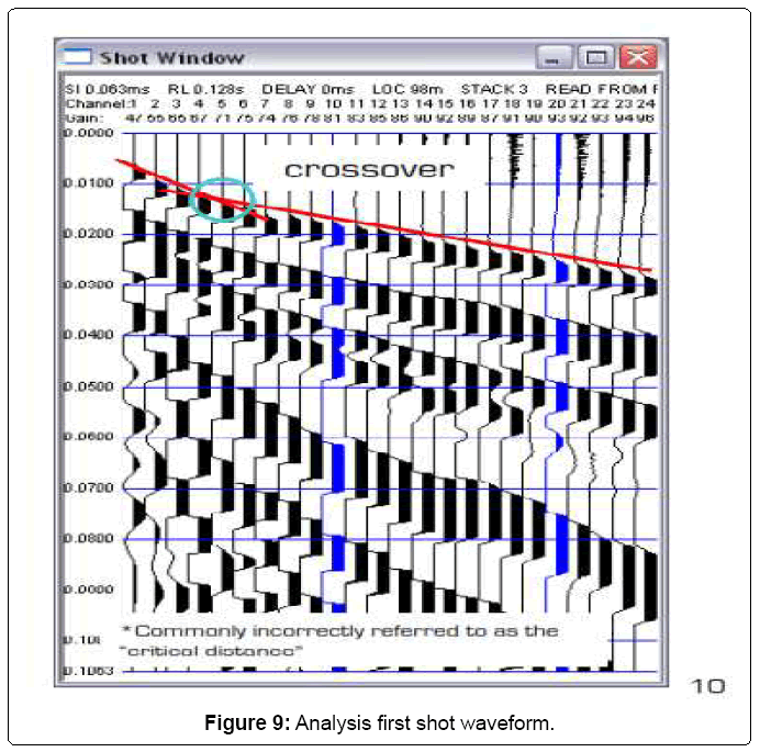
Figure 9: Analysis first shot waveform.
The first shot, the recoded and display in seismograph is shown in Figure 10. The figure show data collected by 24 geophones. The deviation from geophone to other represented the distance between geophone to another. The geophones signal as stairway left direction. The first geophone is the first signals arrive to seismograph, and so on to last geophone is the last signals arrive to seismograph.
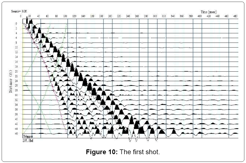
Figure 10: The first shot.
The second shot seismic source located between geophone number 12 and 13 (at middle distance=24 m). In this case the signals from all geophones as triangle shape the head of this triangle at middle. The first geophones reading seismic signal at geophones number 12 and 13, and so on to geophones number 1 and 24, Figure 9 shows the geophones signal.
From Figure 11 it is very clarification the shot at middle distance. Because the time for arriving signals for all two geophones symmetric is constant, so there is symmetric shown in figure.
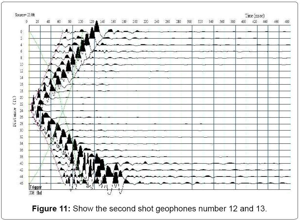
Figure 11: Show the second shot geophones number 12 and 13.
Third shot in third shot the signals are at variance in first shot signals. The seismic source at last geophone (geophone number 24), so the Figure 10 is at variance in Figure 12. The geophone number 24 is the first reading signals and so on until geophone number one. The geophones signal as stairway right direction. Third shot as shown in Figure 10.
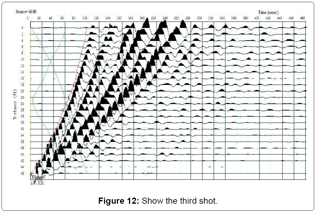
Figure 12: Show the third shot.
Fifth block is software package (seisImager/2D) [10]. The data that collected in seismograph export to P.C. the program make process on this data. The first processing on data, Set the display gain so the first breaks are clearly visible.
Determine the first arriving time. The data consists of a travel time T (sec) for each geophone location X (m). Data used to plot travel time curve. It is use to determine the first arriving time as shown in Figure 13. In this experiment determine by manual technique.
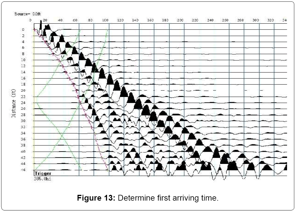
Figure 13: Determine first arriving time.
After determine first arriving time; use time traveling curves to identify subsoil layers. This technique applied by the GRM method according to Palmer (Generalized Reciprocal Method, Palmer, 1981 and 1991). Dromocrones of longitudinal waves are obtaining by analyzing first arrivals of elastic waves (Figure 13).
If we read the geophones data and plot this data we find there is break down, this break down indicate the wave path through another layer as shown in Figure 14 and by using the generalized reciprocal method (GRM) is a technique for delineating undulating refractors at any depth from in line seismic refraction data consisting of forward and reverse travel times [11]. The travel times are used in refractor velocity analysis and time depth calculations.
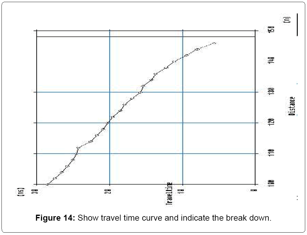
Figure 14: Show travel time curve and indicate the break down.
This results of refractor velocity analysis being the simplest and the time depths showing the most detail. In contrast conventional reciprocal method which has XY equal to zero is especially prone to produce numerous fictitious refractor velocity changes. As well as producing gross smoothing of irregular refractor topography. The depth conversion factor is relatively insensitive to dip angles up to about 20 degrees. As a result, depth calculations to an undulating refractor are particularly convenient even when the overlying strata have velocity gradients. The GRM provides a means of recognizing and accommodating undetected layers provided an optimum XY value can be recovered from the travel time data. The presence of undetected layers can be inferred when the observed optimum XY value differs from the XY value calculated from the computed depth section. The undetected layers can be accommodated by using an average velocity based on the optimum XY value. This average velocity permits accurate depth calculations with commonly encountered velocity contrasts. Reciprocal times are about equal (good quality check). The forward and reverse shots are symmetrical about the center indicating there is little or no dip on refractor. The Generalized Reciprocal Method (GRM) as shown in Figure 15. The GRM method is necessary because dependent on absolute time to inverts from time depth (ms) to depth (m) this method is very sensitive to thickness of slow superficial soil layers [12]. All profiles were interpreted as a two layers configuration. The first layer with velocity of 300-400 m/s corresponds to the superficial soils. The next layer 550-850 m/s to further near surface of mixes sand, these results refer to Table 1 are considered the same results. The same velocities for all layers. Time term inversion gives a quick solution for 2 to 3 layer cases with evident breaks in slope. After we determine the travel time curve the program plot the layers module result. The layers module result plot the detecting layers and velocity in all layers as shown in Figure 16.
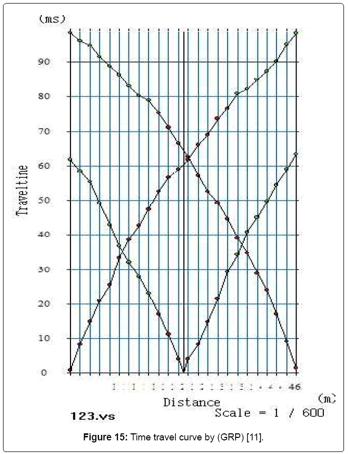
Figure 15: Time travel curve by (GRP) [11].
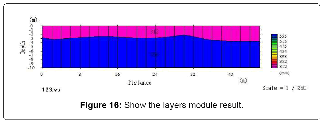
Figure 16: Show the layers module result.
| Material | Velocity Vp m/s |
|---|---|
| 1- Unconsolidated materials | |
| Sand dry | 200-1000 |
| Sand (water-saturated) | 1500-2000 |
| Clay | 1000-2500 |
| Glacial till (water-saturated) | 1500-2500 |
| Permafrost | 3500-4000 |
| 2-Sedimentary rocks | |
| Sandstones | 2000-6000 |
| Tertiary sandstone | 2000-2500 |
| Pennant sandstone (Carboniferous) | 4000-4500 |
| Cambrian quartzite | 5500-6000 |
| Limestone | 2500-6000 |
| Cretaceous chalk | 2000-2500 |
| Jurassic oolites and bioclasticlimestones | 3000-4000 |
| Carboniferous limestone | 5000-5500 |
| Dolomites | 2500-6000 |
| Salt | 4500-5000 |
| Anhydrite | 4500-6500 |
| Gypsum | 2500-3500 |
| 3-Igneous/Metamorphic rocks | |
| Granite | 5500-6000 |
| Gabbro | 6500-7000 |
| Ultramafic rocks | 7500-8000 |
| Serpentinite | 5500-6500 |
| 4-Pore fluids | |
| Air | 300 |
| Water | 1400-1500 |
| Ice | 3400 |
| Petroleum | 1300-1400 |
| 5-Other material | |
| Steel | 6100 |
| Iron | 5800 |
| Aluminum | 6600 |
| Concrete | 3600 |
Table 1:Compressional wave velocities in Earth materials Vp[14,15].
Sixth block is seismogram. From the figure show there are two layers the first layer have thickness almost 3 m. It is as surface layer, and P-waves velocity in this layer is 312 m/s. the second layer have thickness almost 7 m, and P-waves velocity in this layer is 558 m/s [13]. The velocity the subsoil layers give indication about the subsoil layers formations contain, such as sandstone, carbonate [14], gas and oil reservoir and other material. For the Table 1 we have same reading of P-waves velocity for many formations material, the P and S waves velocity (Table 1) are the same velocity in our investigations. S-waves measure by planting horizontal geophone in seismograph studies. It calculated by S-waves equation, it equal 0.7 P-waves velocity [15-17].
Seismology is curtailment as system model. This system model consists of blocks diagram. All blocks have main function. Seismic refraction techniques used in exploration for minerals, subsoil layers petroleum, and subsoil layers water. This study obtained by seismograph. Seismograph is dependent on refraction P-waves. In this work the predicted layers are determined the first layer velocity (p-wave) is 300-400 m/s corresponds to the superficial soils, and velocity in second layer 550-850 m/s to further near surface of mixes sand. P-waves velocity increase with depth increase, Due to increase porosity, density and wetness layers. The seismograph results indicate that the seismic wave’s velocities are equal seismic waves velocity obtains by seismic waves model.