Journal of Geology & Geophysics
Open Access
ISSN: 2381-8719
ISSN: 2381-8719
Research Article - (2014) Volume 3, Issue 2
Committee Machine (CM) or ensemble introduces a machine learning technique that aggregates some learners or experts to improve generalization performance compared to single member. The constructed CMs are sometimes unnecessarily large and have some drawbacks such as using extra memories, computational overhead, and occasional decrease in effectiveness. Pruning some members of this committee while preserving a high diversity among the individual experts is an efficient technique to increase the predictive performance. The diversity between committee members is a very important measurement parameter which is not necessarily independent of their accuracy and essentially there is a tradeoff between them. In this paper, first we constructed a committee neural network with different learning algorithms and then proposed an expert pruning method based on diversity and accuracy tradeoff to improve the committee machine framework. Finally we applied this proposed structure to predict permeability values from well log data with the aid of available core data. The results show that our method gives the lowest error and highest correlation coefficient compared to the best expert and the initial committee machine and also produces significant information on the reliability of the permeability predictions.
Keywords: Committee machine, Genetic algorithm, Ensemble pruning, Permeability
Committee machines (CM) or ensembles are a machine learning method that each of its members can do the same task. The motivation behind introducing the CM is to aggregate a set of experts so that this constructed model improves the generalization performance in comparison to each member alone [1]. Numerous academic and experimental studies have been done in ensemble methods that significantly show that this approach will be effective if their members are both diverse and accurate [1,2]. Diversity between experts is a very important parameter that is not necessarily independent of their accuracy and essentially there is a trade-off between them [3]. In a CM, the expectation is that distinct experts converge to different local minima on the error surface, and the overall output improves the performance [4,5]. Naturally, a CM includes two phases; first, creating individual members and then a combination of output from the created experts. Some authors (Muoz et al. [6], Caruana et al. [7] Fan et al. [8] and Tsoumakas et al. [9]) have considered an additional intermediate phase. The goal of this additional phase is to reduce the CM size before the combination stage, which this is called expert/ensemble pruning. A CM structure with the three mentioned stages is illustrated in Figure 1, whereby it consists of multiple experts and a single combiner. In homogeneous models, the individuals are created from different implementations of the same learning algorithm [1]. Bagging [10] and boosting [11] are two popular homogeneous methods. In heterogeneous models, the individuals are obtained by running different learning algorithms on the same dataset. The last stage of building a CM or ensemble is the combination of techniques. Many investigations have been done to design suitable fusing methods to combine the experts output and produce final result such as; simple averaging [12], majority voting [13], ranking [13,14], weighted averaging [15], fuzzy integrals [16] and weighted majority voting [17]. Several Artificial Intelligence (AI) techniques have been applied by many researchers to predict reservoir oil properties by utilizing conventional well log data. This is due to the expensive cost of traditional prediction methods in oil exploration. Permeability is one of the fundamental and effective reservoir oil properties, which is defined as the ability of porous rock to transmit fluid. A coring method based on rock samples in the laboratory and well tests are direct methods to determine permeability which are costly and time consuming [18]. Data sampling based on coring methods also does not provide a continuous profile along the depth of the formation. Therefore, permeability prediction based on well log data, which is much less costly than direct methods, is a significant research area in petroleum engineering. Several AI techniques such as neural networks, fuzzy logic and committee machines [19-37] have been used for permeability prediction. In this paper, we propose a new framework based on expert pruning on committee neural network to predict permeability in the Ahvaz oil field of Iran.
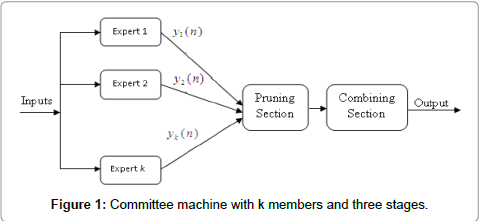
Figure 1: Committee machine with k members and three stages.
As mentioned above, the constructed CMs are sometimes unnecessarily large and introduce some limitations in predictive performance. Therefore, in a full set of experts, maybe there are some weak ones that can have negative effects on overall performance. Pruning some of these members while preserving a high diversity among the experts is an efficient technique for increasing the predictive performance. The benefits of ensemble pruning in improving efficiency and producing predictive performance are well known. In fact, the ensemble pruning problem is similar to an optimization problem, in which the objective is to find the best subset of individuals from the original ensemble. To the best of our knowledge, for a set with T member, there are (2 T−1) subsets, so in the moderate sized ensemble, the exhaustive search becomes intractable. In Zhou et al. [38], the authors presented a pruning approach based on a genetic algorithm named GASEN (Genetic Algorithm based Selective Ensemble). In their method, the individual members with a weight greater than a present threshold (λ) could be selected to join the sub-ensemble and the others are dropped. In Brown et al. [39], the authors proposed a method for managing the diversity based on decomposition of bias-variancecovariance in regression ensembles. They also showed that there is a relationship between the error function and the negative correlation algorithm [40] and this method can be viewed as a framework for application on regression ensembles. Clustering is another approach proposed by Bakker and Heskes [41] for ensemble pruning. In this method, experts are divided into a number of sets according to the similarity of their outputs, and then a single network is selected from each cluster. This method does not guarantee that the selected experts improve the generality prediction of the ensemble, but it is more suitable for qualitative analysis and introduces a new method to ensemble pruning. In Jafari et al. [42], the authors proposed a pruning method based on a genetic algorithm with a new error matrix.
The diagonal elements of the matrix measure individual squared errors while the off-diagonal elements correspond to correlation-like values. Finally, in their method, experts with a weight equal to one are selected as members of the final sub-CM. In this paper, we propose another pruning approach that is based on a diversity and accuracy trade-off based on Rooney’s method [43]. This proposed method is developed for predicting permeability from well log data with the aid of available core data.
In petroleum industry, obtaining an accurate estimation of the hydrocarbon in place before exploration or production stages is the most important objective. Therefore, reliable prediction of reservoir characterization is very helpful for evaluating and designing any development plan for production from the field. The objective of our research is to introduce an intelligent system to predict permeability by utilizing the well log data in an un-cored interval of the same well or in an un-cored well of the same field. In this paper, we will introduce a new intelligent structure named Pruned Committee Neural Network (PCNN) with high accuracy, fast processing and low cost to predict permeability.
Input selection and data preparation
In this study, well logs and core data were collected from the Ahvaz fields of the National Iranian Oil Company (NIOC). The permeability derived core data for this study ranges from 0.002 to 1882.94 millidarcy. This causes complications when assessing the reliable performance in our prediction. To overcome this problem, we normalized it in the range of 0 to 1. Selecting suitable inputs with a stronger relationship to the target data plays an important role in model construction. The relationship between available well log data, which are porosity, neutron (NPHI), density (RHOB), sonic (DT), gamma ray (SGR), photoelectric (PEF), effective porosity (PHIE), formation true resistivity (RT) and normalized core permeability is illustrated in Figure 2. As demonstrated in the figure, five well logs that are shown on the y-axis as input variables have a strong relationship (high correlation coefficient) with permeability as the output variable that is shown on the x-axis. We also have used another method to select stronger input data on the target. For this purpose, we applied the Mallows’ Cp statistic method to obtain the best fit for a regression model that is utilized using a Least Square (LS) algorithm. This method is suitable for feature selection, where a number of independent variables are available to predict certain dependent variables. By utilizing these methods, the NPHI, RHOB, DT, PEF and PHIE are selected as input data to predict permeability.
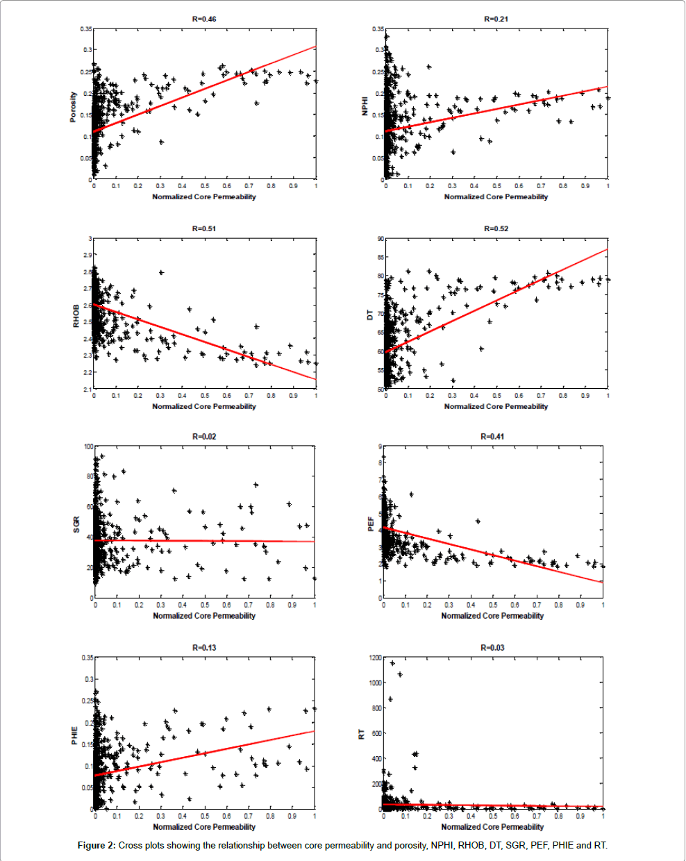
Figure 2: Cross plots showing the relationship between core permeability and porosity, NPHI, RHOB, DT, SGR, PEF, PHIE and RT.
Porosity: Porosity is one of the essential properties of reservoir rocks and defined as a proportion of fluid-filled (oil, gas and water) space found within the rock. It is the fraction of a porous medium that is void space and measured as a fraction and poses no units. Porosity can be classified into two main categories which are; absolute and effective porosity. The first one means, the total porosity of the rock without considering the connections of the voids. Effective porosity means the voids that are interconnected.
Resistivity logs: Resistivity logs can be used to measure the ability of rocks to carry out electrical current such that sand filled with salt water has lower resistivity rather than sand filled with oil or gas. The primary aim of this logging method is to determine hydrocarbon saturation but the other usages of it are to determine porosity, permeability, lithology and fracture zones.
Gamma ray log: This logging tool measures radiation omitted by naturally occurring potassium, thorium, and uranium in formation verses depth. Gamma ray log also known as shale log because the radioactive count in shale is higher than clean sand or carbonates. This logging tool is suitable to determine bed thicknesses, mineral analysis, correlation between wells and etc.
Sonic log: This type of logging is also known as acoustic or velocity log that is widely used for porosity logs to quantitative interpretation of hydrocarbon saturation. This log is based on measuring the sound waves’ speed in travel through 1 m of subsurface formations. This logging tool also is used for many other purposes such as delineate fractures and indicating lithology, determining integrated travel time, secondary porosity, mechanical properties, acoustic impedance, quality of cementation behind the formation and detecting over-pressure.
Density log: Density log is another logging tool to determine porosity especially in shale that reacts to variation of the specific formation gravity. This tool emits neutrons into the rock and measures the back-scattered radiation that is received by the detector in the instrument. Density log can also be used to determine lithology, gas detection, estimating mechanical properties, evaluation of shaly sands and etc.
Neutron log: The third significant tools to determine formation porosity is neutron log. This log has a radioactive source, and measures the reaction energy between emitted and detected neutrons back to the tool. When the emitted neutrons crashed with the hydrogen’s nucleus, the most emitted energy will be lost. Therefore based on the hydrogen index, apparent neutron porosity can be determined. The neutron logs almost in combination with other logs such as density or sonic logs can be used to determine porosity, volume of shale, matrix type, lithology, formation fluid type and etc.
Permeability: Permeability is one of the fundamental and effective reservoir properties which are defined as the ability of porous rock to transmit fluid. It is commonly measured in darcy (d) or millidarcy (md). Permeability can be obtained by direct and indirect methods. Coring method based on rock samples in laboratory and well tests are direct methods and indirect methods are based on well logs data [18]. The data sampling based on coring methods does not provide a continuous profile along the depth of the formation. However, the two mentioned direct methods provide the most reliable permeability values of a formation but they are costly and time-consuming. Therefore, permeability prediction based on well logs data which are much less costly compared to direct methods is a significant research area in petroleum engineering. Intelligent techniques are suitable research methods in petroleum engineering because finding an explicit relation between rock permeability and well log data parameters are impossible.
Creating the CM members
The first step of the method is to build a set of ten experts based on Feed Forward Neural Networks (FFNN) with different training algorithms. All of these algorithms use a back propagation technique to adjust the weights for getting the optimum performance, which is usually minimum MSE. For this purpose, we employed ten highperformance algorithms that converged faster than the others. They are variable learning rate BPNN (GDA, GDX), resilient BPNN (RP), Conjugate Gradient (CGF, CGP, CGB, and SCG), Quasi-Newton (BFG, OSS) and Levenberg-Marquardt (LM). The numbers of neurons in input and output layers are exactly equal to the number of inputs and outputs parameters respectively. However, the number of neurons in hidden layers depends on the problem in hand which in our study obtained by trial and error processes to get the best performance based on MSE and R2. Finally, the best architecture is selected as 5-X-1 for permeability prediction. The symbol X means the different number of neuron in hidden layer for different training algorithm. The value 5 means the number of input layer and 1 means the number of output layer in NN. The other important parameter that we had to determine before training the networks was the stopping criteria. During the training of a neural network, over fitting problem may occur. It indicates that, MSE is very small for training data and is very high for the new (test) data (i.e., previously unseen data). This means that, the network has memorized the training data and could not learn how to generalize to new situations. There are some ways to overcome the cover fitting problem such as using large enough networks, increase the size of the training set, regularization and early stopping [44]. The early stopping is a default generalization method for the multilayer FFN in the Matlab neural network toolbox. In this method, the data samples are divided into three sets, which are training, validation and test sets. In each epoch of the training process, the MSE on the validation set is monitored and will be stopped when the validation error increases. The training sets are required for updating the weight between the connected neurons in all layers. Moreover, the testing sets are used to test how successfully the network learned to predict the new data, which are not used during the learning process.
Expert pruning
The constructed CMs are sometimes unnecessarily large and provide some shortcomings in the model which requires extra memory, a high computational cost and sometimes has negative effects on overall performance due to the weak predictive performances of some experts. One of the significant methods to reduce the mentioned limitation in a CM is to prune the committee members. Expert pruning, while preserving a high diversity among the individual members, is an efficient technique for increasing the predictive performance. In this stage, we used an equation that considers both accuracy and diversity. Assume D ={(xn, yn ); n =1,2,...,N} is the training data and the generated error for the j-th individual member based on the n-th input is set to Ej (xn ). The error function can be any differentiable function suitable to the problem domain such as squared error or absolute error. Therefore, the total error of the j-th member is calculated by equation (1), whereas equation (2) selects the expert with the minimum error among all K predictors.
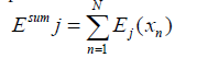 (1)
(1)
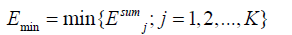 (2)
(2)
Finally, the accuracy of the l-th expert can be defined by equation (3).
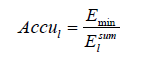 (3)
(3)
To determine the diversity, we calculated the correlation between El and Ej as below; If corre(El ,Ej ) > λ for all l ≠ j , then we increase the value of the counter C by one unit and finally the total diversity of the l-th expert can be defined as equation (4).
Divl (N-C)/N for l= 1,…, K (4)
Where λ є (0,1) is a user-defined constant value. Finally, we defined the l-th output of the ensemble by Fl (x) as Equation (5).
Fl (x)=(1-α)Accul Divl for l = 1,2,…,K (5)
The pruning strategy is based on selecting k individuals of the K networks, which have the highest values of Fl (x), where α is ranged from 0 to 1 with a step size equal to 0.05.
Combination stage
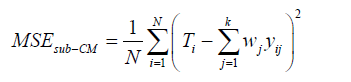
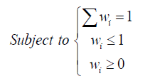
After obtaining the optimum subset of experts, we have to combine them with an efficient method. In this paper, we have used the generalized reduced gradient (GRG) nonlinear method from MSExcel to obtain the optimal weight for each expert by minimizing the mean square error function (equation 6). This algorithm finds the best solution by searching over all the feasible areas that is created by the defined constraints which are shown in equation (7).
 (6)
(6)
 (7)
(7)
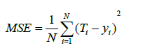
where yij is the output of the j-th expert based on the i-th input, Ti is the target value for the i-th input, and N is the number of data points. In this paper we have used two evaluation measures to compare the performance of different techniques, namely the correlation coefficient (R2) and MSE, which are defined in equations (8) and (9) respectively. The correlation coefficient is a quantity that gives the quality of a least squares fitting between two original data T and Y (equation 9).
 (8)
(8)
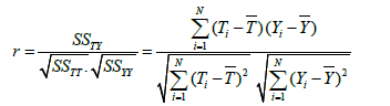 (9)
(9)
The original data (917 data points) were divided into a training set (550 samples), validation set (183 samples) and testing set (184 samples) for the whole of the training algorithms. After a few retraining iterations, the best performances were selected for each method and finally utilized for test data to predict our target, which was based on the value of MSE and R2. The results of testing data for all experts to predict permeability are shown in Figure 3 and Table 1. As shown in the Table 1, about seven experts have R2 greater than 0.9 and MSE less than 0.0015, that it means a very good performance for permeability prediction. By comparing the implementation results listed in the table, the lowest MSE and highest R2 are obtained using the Broyden-Fletcher- Goldfarb-Shanno Quasi-Newton (BFG) algorithm. The values of Fl (x), as mentioned in equations (1)-(5), for all experts based on testing data with different α are calculated and illustrated in Table 2. The value of λ is obtained by using a trade-off between accuracy and diversity and is considered equal to 0.6. There are two main approaches in literature related to the size of the final sub-CM. The methods are fixed percentage size and dynamic selection. The first one will be defined by the user, and the second one is based on the predictive performance of the different subsets that were encountered during the search process from the first to last of the individual members. In this study, we applied the proposed method for fixed predefined k members that started from one and the other experts are added sequentially until the predictive performance starts to decrease. By applying this technique, the best performance obtained is by k=3 for permeability prediction, which is about thirty percent of the total experts. Figure 4, shows MSE and R2 values of predicted permeability based on the different learning algorithms. Three highest values for each Fl (x) related to ten training algorithms are selected and marked in Table 2 with gray color. As demonstrated in the table, three sub-CMs have the highest value of Fl (x). The first sub- CM includes (BFG, CGB and RP) for 0 ≤ α ≤ 0.2. The second sub-CM includes (BFG, LM and RP) for 0.25 ≤ α ≤1. Finally, the third sub-CM includes (BFG, GDA and RP) or (GDA, LM and RP) for α=1. The final weight for four mentioned sub-CMs is calculated based on the GRG nonlinear method mentioned in section 3.4. Then each expert has a weight value, and the output of the sub-CM is obtained by equation (10).
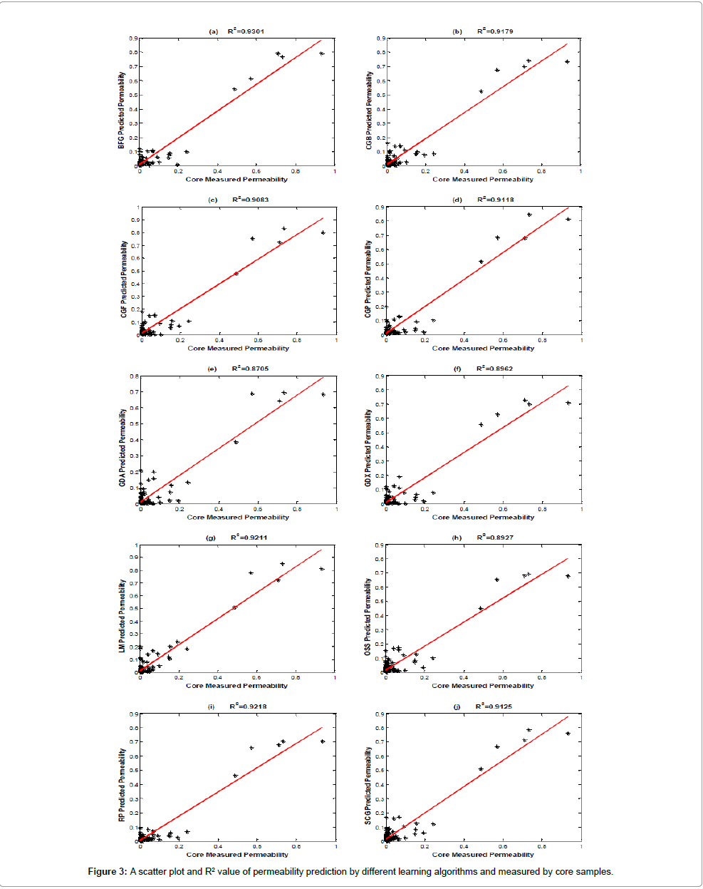
Figure 3: A scatter plot and R2 value of permeability prediction by different learning algorithms and measured by core samples.
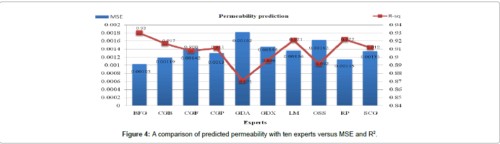
Figure 4: A comparison of predicted permeability with ten experts versus MSE and R2.
| Experts | BFG | CGB | CGF | CGP | GDA | GDX | LM | OSS | RP | SCG |
| R2 | 0.93 | 0.918 | 0.908 | 0.912 | 0.872 | 0.896 | 0.921 | 0.893 | 0.922 | 0.912 |
| MSE | 0.001 | 0.0012 | 0.0014 | 0.0013 | 0.0018 | 0.0015 | 0.0014 | 0.0016 | 0.0012 | 0.0013 |
Table 1: Performance of different learning algorithms to predict permeability individually.
| Alpha | BFG | CGB | CGF | CGP | GDA | GDX | LM | OSS | RP | SCG |
| 0 | 1 | 0.8658 | 0.7237 | 0.7904 | 0.5644 | 0.7022 | 0.7532 | 0.6337 | 0.8925 | 0.7626 |
| 0.05 | 0.96 | 0.8275 | 0.6926 | 0.7559 | 0.5462 | 0.6771 | 0.7405 | 0.607 | 0.8579 | 0.7295 |
| 0.1 | 0.92 | 0.7892 | 0.6614 | 0.7213 | 0.528 | 0.652 | 0.7279 | 0.5803 | 0.8232 | 0.6964 |
| 0.15 | 0.88 | 0.751 | 0.6302 | 0.6868 | 0.5098 | 0.6269 | 0.7152 | 0.5536 | 0.7886 | 0.6632 |
| 0.2 | 0.84 | 0.7127 | 0.599 | 0.6523 | 0.4916 | 0.6018 | 0.7026 | 0.5269 | 0.754 | 0.6301 |
| 0.25 | 0.8 | 0.6744 | 0.5678 | 0.6178 | 0.4733 | 0.5766 | 0.6899 | 0.5003 | 0.7194 | 0.597 |
| 0.3 | 0.76 | 0.6361 | 0.5366 | 0.5833 | 0.4551 | 0.5515 | 0.6772 | 0.4736 | 0.6847 | 0.5638 |
| 0.35 | 0.72 | 0.5978 | 0.5054 | 0.5487 | 0.4369 | 0.5264 | 0.6646 | 0.4469 | 0.6501 | 0.5307 |
| 0.4 | 0.68 | 0.5595 | 0.4742 | 0.5142 | 0.4187 | 0.5013 | 0.6519 | 0.4202 | 0.6155 | 0.4976 |
| 0.45 | 0.64 | 0.5212 | 0.4431 | 0.4797 | 0.4004 | 0.4762 | 0.6393 | 0.3935 | 0.5809 | 0.4644 |
| 0.5 | 0.6 | 0.4829 | 0.4119 | 0.4452 | 0.3822 | 0.4511 | 0.6266 | 0.3668 | 0.5462 | 0.4313 |
| 0.55 | 0.56 | 0.4446 | 0.3807 | 0.4107 | 0.364 | 0.426 | 0.6139 | 0.3402 | 0.5116 | 0.3982 |
| 0.6 | 0.52 | 0.4063 | 0.3495 | 0.3762 | 0.3458 | 0.4009 | 0.6013 | 0.3135 | 0.477 | 0.3651 |
| 0.65 | 0.48 | 0.368 | 0.3183 | 0.3416 | 0.3276 | 0.3758 | 0.5886 | 0.2868 | 0.4424 | 0.3319 |
| 0.7 | 0.44 | 0.3297 | 0.2871 | 0.3071 | 0.3093 | 0.3507 | 0.576 | 0.2601 | 0.4077 | 0.2988 |
| 0.75 | 0.4 | 0.2915 | 0.2559 | 0.2726 | 0.2911 | 0.3255 | 0.5633 | 0.2334 | 0.3731 | 0.2657 |
| 0.8 | 0.36 | 0.2532 | 0.2247 | 0.2381 | 0.2729 | 0.3004 | 0.5506 | 0.2067 | 0.3385 | 0.2325 |
| 0.85 | 0.32 | 0.2149 | 0.1936 | 0.2036 | 0.2547 | 0.2753 | 0.538 | 0.1801 | 0.3039 | 0.1994 |
| 0.9 | 0.28 | 0.1766 | 0.1624 | 0.169 | 0.2364 | 0.2502 | 0.5253 | 0.1534 | 0.2692 | 0.1663 |
| 0.95 | 0.24 | 0.1383 | 0.1312 | 0.1345 | 0.2182 | 0.2251 | 0.5127 | 0.1267 | 0.2346 | 0.1331 |
| 1 | 0.2 | 0.1 | 0.1 | 0.1 | 0.2 | 0.2 | 0.5 | 0.1 | 0.2 | 0.1 |
Table 2: The values of Fl (x) and α for all networks with different training algorithms.
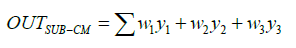 (10)
(10)
Table 3 and Figure 5 show a comparison between the results of the best expert (BFG) with lowest MSE and highest R2, four obtained sub- CMs and the full CM with ten experts for permeability prediction. As demonstrated in the table, the second obtained sub-CM introduces the highest R2 and lowest MSE compared to others. The final weights for the three individual members of this pruned CM were 0.427, 0.322 and 0.251 for BFG, LM, and RP respectively.
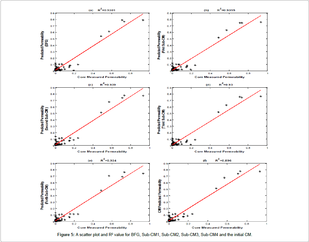
Figure 5: A scatter plot and R2 value for BFG, Sub-CM1, Sub-CM2, Sub-CM3, Sub-CM4 and the initial CM.
| Algorithm | BFG | First -CM | Second - CM | Third -CM | 4th -CM | Initial CM |
| R2 | 0.93 | 0.931 | 0.939 | 0.93 | 0.934 | 0.939 |
| MSE | 0.001 | 0.00099 | 0.00089 | 0.001 | 0.00094 | 0.00089 |
Table 3: A comparison between the best experts, four obtained sub-CM and initial CM.