Journal of Information Technology & Software Engineering
Open Access
ISSN: 2165- 7866
ISSN: 2165- 7866
Research - (2019)Volume 9, Issue 2
The paper goes over what would happen when deep learning methods are implemented for University Network Traffic. In order to predict the outcome, the paper will compare the network before the implementation of deep learning and after the implementation of deep learning. If the results show an increase in data transfer speed after the implementation of deep learning, it suggests that the implementation of deep learning in any network system will most likely improve the data transfer speed. The paper first defines what deep learning is. It then utilizes different methods of deep learning in order to train the system. The system will go through the training phase, testing phase, and the prediction phase in order to familiarize it with the current network system. Once it understands the network system, it will find the optimized network system in order to improve the speed of network connection.
Network traffic; Communication technology; Information system; Regression analysis
In the past, most universities have network traffic of information & communication technology center in all the faculties, institutes and units. Nowadays, most universities have implemented more web-based applications in order to support the academician and administrative activities in the teaching-learning process. These activities include financial information systems, human resources information system, academic information systems, e-library, e-learning, etc. A good internet traffic regulation is required to support these web-based applications. This traffic regulation can be achieved by predicting the university network traffic using the past network traffic data.
Currently, some common prediction methods that have been broadly implemented are the simple method regression analysis, decomposition, and exponential smoothing method. Though these methods are very well implemented in some predictions, they still have some drawbacks. A linear data can be predicted very well using these methods, but for non-linear data, the results are less accurate and they also can’t be applied to predict data that uses many factors [1]. However, predicting using the artificial neural network (ANN) model can give better results, and it is also very effective for predicting [2], in which, this method is found capable to work well on the non-linear time-series data. Therefore, this tutorial paper will implement one of the artificial neural network models, namely the deep neural network model to predict the university network traffic using the past network traffic data.
Basics of deep learning
Deep learning is an active research area in the fields of artificial intelligence and machine learning. Deep learning has been proven to be the most effective approach for solving many complicated real-world problems like prediction, object recognition, natural language processing, speech and audio processing, information retrieval, multi-modal and multi-task learning, etc.
Definitions of deep learning
Deep learning has different closely related definitions. Necessary definitions of deep learning are as follows.
Definition 1: Deep learning is a class of machine learning techniques that is mainly used for pattern analysis and classification.
Definition 2: Deep learning is a set of algorithms in machine learning that try to learn in multiple levels where each level is learning features or representations at increasing levels of abstraction. It normally uses artificial neural network models having more than one hidden layer.
Definition 3: Deep learning is a new area of machine learning research, introduced with the aim of moving machine learning nearer to at least one of its original goals: Artificial Intelligence.
Why does deep learning work?
Deep learning works due to the following reasons:
The brain performs many levels of processing. Each level is the learning options or representations at increasing levels of abstraction. For example, the brain first extracts edges, then patches, surfaces, objects, etc., according to the standard model of the visual cortex. This study has inspired the researchers to develop deep learning models. Deep learning models attempt to mimic the working of the brain. They have more than one hidden layer for information processing- same as the brain.
Shallow architectures work well in solving many simple or wellconstrained problems, but they do not work well in solving complicated real-world problems like object recognition, natural language processing, speech processing, etc., because of their limited depth and representational power. But deep learning models work well in solving complicated real-world problems because of their deep architectures (more than one hidden layer) and representational power.
Types of deep learning networks
Two types of deep learning networks are explained as follows.
Supervised deep learning networks
Supervised deep learning networks [3] are used for supervised learning tasks. They are also called discriminative deep learning networks. In supervised learning tasks, both input observations and output observations are given. During the learning phase, supervised deep learning networks try to find the connections between two given observations, namely inputs and outputs. These learned connections in form of weights can predict the outputs of new input observations that have not been previously learned.
Unsupervised deep learning networks
Unsupervised deep learning networks [3] are used for unsupervised learning tasks. They are also called generative deep learning networks. In unsupervised learning tasks, all input observations are given and no output observations are available. Unsupervised deep learning networks try to find the associations and patterns among input observations.
Deep neural network
We will use the deep neural network [4] to predict the university network traffic using past network traffic data. Deep neural network is a supervised deep learning network. Deep neural network is a neural network that has two or more hidden layers. The architecture of deep neural network is shown in Figure 1.

Figure 1: Architecture of deep neural network.
The leftmost layer of the network is known as the input layer. X1, X2 and X3 are inputs of the network. The rightmost layer of the network is called the output layer. Y1 is an output of the network. The middle layer of the network is called the hidden layer. It is called the hidden layer because its values are not observed in the training samples. The network is comprised of one input layer, two hidden layers and one output layer. The network has 3 input units, 5 hidden units, 1 output unit. Node B1 represents 3 bias values, node B2 represents 2 bias values and node B3 represents 1 bias value. Bias values represented by node B1, B2 and B3 might be different. So, the network has a total of 6 bias units. The convention used for weights and bias is as follows:
WX1-H11 denotes the value of weight associated with the connection between unit X1 and unit H11.
BB1-H11 denotes the value of bias associated with the connection between unit B1 and unit H11. The activation function is denoted by f. The computation represented by this network is given as follows.
H11=f (X1WX1-H11 + X2WX2-H11 + X3WX3-H11 + BB1-H1)
H12=f (X1WX1-H12 + X2WX2-H12 + X3WX3-H12 + BB1-H12)
H13=f (X1WX1-H13 + X2WX2-H13 + X3WX3-H13 + BB1-H13)
H21=f (H11WH11-H21 + H12WH12-H21 + H13WH13-H21 + BB2-H21)
H22=f (H11WH11-H22 + H12WH12-H22 + H13WH13-H22 + BB2-H22)
Y1=f (H21WH21-Y1 + H22WH22-Y1 + BB3-Y1)
The network has only two hidden layers so the standard learning strategy is as follows.
1. Randomly initialize the weights of the network.
2. Apply gradient descent using back-propagation.
This kind of network is useful if we are interested in predicting the output.
Back-propagation algorithm for the prediction of the university network traffic
The following back-propagation algorithm [5] can be used to train the deep neural network. The trained deep neural network can then be used to predict the university network traffic.
Given: A set of input-output vector pairs.
Compute: A set of weights that maps inputs onto corresponding outputs.
Step 1: Let A be the number of units in the input layer, as determined by the length of the training input vectors. Let C be the number of units in the output layer. Now choose B, the number of units in the hidden layer. The input and hidden layers each have an extra unit used for bias. The units in the input and hidden layers will sometimes be indexed by the ranges (0,…,A) and (0,…,B). We denote the activation levels of the units in the input layer by xj, in the hidden layer by hj, and in the output layer by oj. Weights connecting the input layer to the hidden layer are denoted by w1ij, where the subscript i is the indexes of the input units and j is the indexes of the hidden units. Likewise, weights connecting the hidden layer to the output layer are denoted by w2ij, where the subscript i is the indexes of the hidden units and j is the indexes of the output units.
Step 2: Initialize the weights in the network. Each weight should be set randomly to a number between -10.0 and 10.0.
w1ij=random(-10.0,10.0) for all i=0,…,A j=1,…,B
w2ij=random(-10.0,10.0) for all i=0,…,B, j=1,…,C
Step 3: Initialize the activations of the bias units. The values of these bias units should never change.
x0=1.0
h0=1.0
Step 4: Choose an input-output pair. Suppose the input vector is xi and the target output vector is yi. Assign activation levels to the input units.
Step 5: Propagate the activations from the units in the input layer to the units in the hidden layer using the following activation function.
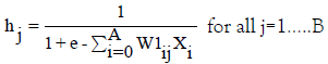
Note that i ranges from 0 to A. w10j is the bias weight for hidden unit j. x0 is always 1.0.
Step 6: Propagate the activations from the units in the hidden layer to the units in the output layer using the following activation function.
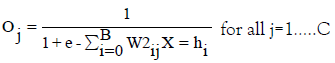
Here, w20j is the bias weight for output unit j. h0 is always 1.0.
Step 7: Compute the errors of the units in the output layer, denoted δ2j. Errors are based on the network’s actual output (oj) and the target output (yj).

Step 8: Compute the errors of the units in the hidden layer, denoted as δ1j.
δ1j=hj (1 - hj) ΣC δ2i * w2ji for all j=1…..B
Adjust the weights between the hidden layer and the output layer. The learning rate is denoted as n; its function is the same as in perceptron learning. A reasonable value of n is 0.05.
Δ w2ij=n * δ2j * hi for all i=0…..B, j=1…..C
Step 10: Adjust the weights between the input layer and the hidden layer.
Δ w1ij=n * δ1j * xi for all i=0…..A, j=1…..B
Step 11: Go to step 4 and repeat. When all the input-output pairs have been presented to the network, one epoch has been completed. Repeat steps 4 to 10 for as many epochs as desired. The above algorithm is for one input layer, one hidden layer and one output layer. However, the above algorithm generalizes straightforwardly to networks of more than one hidden layer. For each extra hidden layer, insert a forward propagation step between steps 6 and 7, an error computation step between steps 8 and 9, and a weight adjustment step between steps 10 and 11. Error computation for hidden units should use the equation in step 8, but with i ranging over the units in the next layer, not necessarily the output layer. The speed of learning can be increased by modifying the weight modification steps 9 and 10 to include a momentum term α. If α is set to 0.01 or so, learning speed is improved.
Phases of deep neural network to predict university network traffic
For prediction of the university network traffic, the deep neural network goes through the following three phases.
Training phase (Learning phase)
Deep neural network uses the pair of input and output values during the learning phase. During the learning phase [6], deep neural network tries to find the connections between the values of inputs and outputs. These learned connections in form of weights can predict the outputs of new inputs that have not been previously learned.
Testing phase
Once the training phase has been successfully completed, we can test the accuracy of the deep neural network in the testing phase. Again, we know the values of all inputs and outputs in the testing phase. In the testing phase [6], we will compare the predicted output value and target output value in order to test the accuracy of the trained deep neural network.
Prediction phase
Once the training and testing phase has been successfully completed, we can use the deep neural network to predict the outputs of new inputs that have not been previously learned.
Application domains of deep learning
This section presents domains in which deep learning methods can be successfully applied.
Prediction (forecasting)
Prediction [7] is the first area in which the application of deep learning methods has been found to be very successful at an industrial scale. Time is the only moving thing in the world that never stops. In the case of forecasting, the human mind is known to be more inquisitive as we know that things change with time. Therefore, we are concerned to make forecasts early. Anywhere time is an influencing factor, there is a hypothetically valuable thing that can be foreseen.
Different types of forecasting we can make the deep learning methods do in real life. Business forecasting assists in forecasting/ predicting the future values of a critical field which has a possible business value in the industry. Deep learning hierarchical decision models can successfully solve the problems in financial prediction and classification [8]. Deep learning can be successfully used to predict the university network traffic, internet traffic, vehicles traffic on highways, the health condition of a person, results of a sport or performance parameters of a player based on previous performances and previous data, weather, earthquakes, rainfall, fog at airport, water quality, crypto-currency prices, stock market returns, human work efficiency in noisy environment, propagation path loss for mobile communications systems, fabrics’ extensibility, etc.
Speech and audio processing
Speech recognition is the second area in which the application of deep learning techniques has been found to be very successful at an industrial scale. The credit of this success goes to the Microsoft research department that initiated the research, forming a close group of academic- industrial researchers to satisfy the industrial need for large-scale development [9].
Speech recognition has been dominated by the Gaussian mixture model - hidden Markov model system long time in the past. Neural networks were a popular approach but they had not been competitive with the Gaussian mixture model - hidden Markov model system. Deep learning and the deep neural networks have started creating their influence in speech recognition after close collaborations between the academic and industrial researchers in 2010. The following two factors quickly spread the success of deep learning in speech recognition to the speech industries.
1. Deep learning techniques have significantly lowered errors compared to the Gaussian mixture model - hidden Markov model system.
2. Strong modelling power of deep neural network has reduced system complexity.
By 2013, the success of deep neural networks has been experimentally confirmed by major speech recognition groups such as Microsoft, Google and IBM, etc.
Deep learning has also quite impacted their power in the area of audio and music processing. Deep learning has mainly impacted music signal processing and music information retrieval in the general field of audio and music processing. A unique set of challenges should be faced by deep learning in these areas. Music audio represents time series signals. Events are prearranged in musical time instead of real time. Musical audio signals change as a function of rhythm and expression. The measured signals usually mix multiple voices that are synchronized in time. Frequency overlapping is also present in mix multiple voices. Musical tradition, composer, style and interpretation are some of the influencing factors. The signal representation problems are higher because of the high complexity and variety of signal. The signal representation problems are well-suited to the high levels of abstraction afforded by deep learning.
The extent of deep learning work in the area of audio and music processing is comparatively less than the extent of work in the area of speech recognition. Much more deep learning work is expected in the area of audio and music processing in the near future.
Object recognition in computer vision
Tremendous progress has been made in applying deep learning techniques in object recognition field of computer vision in the past five years. Computer vision community has accepted the success of deep learning in this area [9]. It is the third area after the speech recognition area in which deep learning methods have been successfully applied.
The features such as scale invariant feature transform (SIFT) and histogram of oriented gradients (HOG) were used for object recognition in computer vision over the past many years. SIFT and HOG only capture low-level edge information. It is much more difficult for the design of features which can effectively capture mid-level information such as edge intersections and/or high-level representation such as object parts. Deep learning automatically learn hierarchies of visual features in both unsupervised and supervised way directly from data to overcome such challenges. The deep learning techniques applied to computer vision field by past researchers are as follows.
1. Unsupervised feature learning: The deep learning is used to extract features only. Extracted features may be subsequently fed to a relatively simple machine learning algorithm for classification or other tasks.
2. Supervised learning: The deep learning is used jointly for feature extraction and classification when large amounts of labelled training examples are available.
Language modeling and natural language processing
The goal of language modeling is to provide a probability of any arbitrary sequence of words or other linguistic symbols such as letters, characters, etc. Natural language processing deals with sequences of words or other linguistic symbols, but the tasks involved in natural language processing are much more diverse than the tasks involved in language modeling. Tasks involved in natural language processing are natural language understanding, generation, translation, parsing, text classification, etc. Thus, natural language processing does not focus on providing probabilities of linguistic symbols. The connection is that language modeling is often an important and very useful component of natural language processing systems.
Deep learning research communities are active when applying deep learning techniques in the field of natural language processing [9]. Natural language processing research community has also considered deep learning as one of the most promising techniques. However, the extent of deep learning work in the area of natural language processing is comparatively less than the extent of its work in the area of speech and vision because the hard proof which proves that deep learning is better than the current state of the art natural language processing methods has not been as strong as available in the area of speech and vision.
Information retrieval
The automated computer system that contains a collection of many documents can be used for the purpose of information retrieval. The goal of information retrieval is to get a set of most relevant documents based on user query [9]. Information needed by a user can be represented by a query. One example of a query is a search string entered in the web search engine. A query may not uniquely identify a single document in the collection but a query may match with several documents with different degrees of relevancy.
A document may include information in the form of text, image, audio and video. Sometimes, a document is called an object in a more general term. Documents often are not saved directly in the information retrieval system. Rather, the system represents them by metadata. Typical information retrieval systems calculate a numeric score of each document indicating how well each document matches with the query and then rank the documents according to this score. Then the systems show the top-ranking documents to the user. If the user wants to refine the query, then the process may be repeated.
Use of deep learning techniques in information retrieval field has just started. The deep learning techniques are mainly used for extracting semantically meaningful features. Extracted semantically meaningful features will be used to rank the documents. Much more deep learning work is expected in the area of information retrieval in the near future.
Multi-modal and multi-task learning
Multi-task learning is a machine learning approach that uses a shared representation to solve several related problems at the same time. There are two major classes of transfer learning. One of them is multi-task learning which focuses on generalizations across distributions, tasks or domains. The other major class is adaptive learning where knowledge transfer is executed in a sequential manner, usually from a source task to a target task. Multi-modal learning is a closely related concept to multi-task learning. In multimodal learning, the learning tasks cut across several modalities for human-computer interactions. Relating information from multiple sources is also involved in multi-modal learning.
Deep learning is used to automate the process of learning effective features or representations for any machine learning task. The deep learning can also be used for automatically transferring knowledge from one task to another concurrently. Multi-task learning is often applied to situations where no or very few training examples are available for the target task domain. So, it is sometimes called zero-shot or one-shot learning. It is obvious that difficult multitask learning naturally fits with the concept of deep learning or representation learning. The shallow learning models were used for multi-modal and multi-task learning before deep learning models were adopted. The reported performance of shallow models was worse than the expected performance. Ultimately, difficult multimodal learning problems have been successfully solved by deep learning models which enable a wide range of practical applications of deep learning models in these areas [9].
Input network traffic data of university
The following Table 1 represents the network traffic data of university for Monday.
Table 1: Network traffic data of a university on Monday.
| Time slot | Input neurons | Output neuron | ||
|---|---|---|---|---|
| P1=Traffic of 5 Feb 2018 |
P2=Traffic of 12 Feb 2018 |
P3=Traffic of 19 Feb 2018 |
P=Traffic of 26 Feb 2018 |
|
| 10:00 am to 10:29 am | 60 Mbps | 62 Mbps | 60 Mbps | 61 Mbps |
| 10:30 am to 10:59 am | 65 Mbps | 70 Mbps | 70 Mbps | 72 Mbps |
| 11:00 am to 11:29 am | 60 Mbps | 65 Mbps | 70 Mbps | 65 Mbps |
| 11:30 am to 11:59 am | 70 Mbps | 70 Mbps | 75 Mbps | 72 Mbps |
| 12:00 pm to 12:29 pm | 80 Mbps | 85 Mbps | 90 Mbps | 75 Mbps |
| 12:30 pm to 12:59 pm | 85 Mbps | 75 Mbps | 75 Mbps | 80 Mbps |
| 1:00 pm to 1:29 pm | 90 Mbps | 90 Mbps | 85 Mbps | 85 Mbps |
| 1:30 pm to 1:59 pm | 85 Mbps | 85 Mbps | 85 Mbps | 80 Mbps |
| 2:00 pm to 2:29 pm | 70 Mbps | 60 Mbps | 70 Mbps | 65 Mbps |
| 2:30 pm to 2:59 pm | 60 Mbps | 70 Mbps | 60 Mbps | 75 Mbps |
| 3:00 pm to 3:29 pm | 60 Mbps | 65 Mbps | 65 Mbps | 55 Mbps |
| 3:30 pm to 3:59 pm | 60 Mbps | 55 Mbps | 55 Mbps | 60 Mbps |
| 4:00 pm to 4:29 pm | 50 Mbps | 50 Mbps | 55 Mbps | 55 Mbps |
| 4:30 pm to 5:00 pm | 60 Mbps | 50 Mbps | 55 Mbps | 55 Mbps |
A University starts at 10:00 am and ends at 5:00 pm. The first column of Table 1 represents 30 minutes time slots between 10:00 am and 5:00 pm. Maximum university network traffic is 90 Mbps and minimum university network traffic is 50 Mbps as per Table 1. In Table 1, P1=Traffic of 5 Feb 2018, P2=Traffic of 12 Feb 2018, P3=Traffic of 19 Feb 2018 and P=Traffic of 26 Feb 2018. The following days (5 Feb 2018, 12 Feb 2018, 19 Feb 2018 and 26 Feb 2018) fall on Monday. So Table 1 represents the network traffic data of university for Monday. Similarly, we can create the network traffic data of a university for Tuesday, Wednesday, Thursday, Friday and Saturday, to predict the university network traffic for the corresponding days. As per the first entry of Table 1, if values of P1=60 Mbps, P2=62 Mbps and P3=60 Mbps, then the value of P would be 61 Mbps. The values of P1, P2 and P3 represent input neurons and the value of P represents output neuron of deep neural network. Here, the university network traffic was measured in Mbps unit.
Normalization process should be performed on the data of Table 1 in order to make training faster and reduce the chances of getting stuck in local optima. The normalized value of the university network traffic can be calculated by using the following equation.
Normalized value of university network traffic=(Actual value of university network traffic – minimum value of university network traffic)/(maximum value of university network traffic – minimum value of university network traffic)
Let us convert P1=60 Mbps into normalized value. Normalized value of P1=(60 – 50)/(90 – 50)=0.25. Similarly, we can convert all the values of Table 1 into the normalized values. The following Table 2 represents the Table 1 in the normalized form. Table 2 can be used to train the deep learning method. The normalization process used in this paper is similar to the normalization process used [10] and other various research papers.
Table 2: Network traffic data of university for Monday in the normalized form
| Time slot | Input neurons | Output neuron | ||
|---|---|---|---|---|
| P1=Traffic of 5 Feb 2018 |
P2=Traffic of 12 Feb 2018 |
P3=Traffic of 19 Feb 2018 |
P=Traffic of 26 Feb 2018 |
|
| 10:00 am to 10:29 am | 0.25 | 0.3 | 0.25 | 0.275 |
| 10:30 am to 10:59 am | 0.375 | 0.5 | 0.5 | 0.55 |
| 11:00 am to 11:29 am | 0.25 | 0.375 | 0.5 | 0.375 |
| 11:30 am to 11:59 am | 0.5 | 0.5 | 0.625 | 0.55 |
| 12:00 pm to 12:29 pm | 0.75 | 0.875 | 1 | 0.625 |
| 12:30 pm to 12:59 pm | 0.875 | 0.625 | 0.625 | 0.75 |
| 1:00 pm to 1:29 pm | 1 | 1 | 0.875 | 0.875 |
| 1:30 pm to 1:59 pm | 0.875 | 0.875 | 0.875 | 0.75 |
| 2:00 pm to 2:29 pm | 0.5 | 0.25 | 0.5 | 0.375 |
| 2:30 pm to 2:59 pm | 0.25 | 0.5 | 0.25 | 0.625 |
| 3:00 pm to 3:29 pm | 0.25 | 0.375 | 0.375 | 0.125 |
| 3:30 pm to 3:59 pm | 0.25 | 0.125 | 0.125 | 0.25 |
| 4:00 pm to 4:29 pm | 0 | 0 | 0.125 | 0.125 |
| 4:30 pm to 5:00 pm | 0.25 | 0 | 0.125 | 0.125 |
Coding snapshots
The following code divides the university network traffic data into training and testing data set.
static void DivideTrainTest(double[][] alltheData, double TrainPrediction, int seed, out double[][] trainDataSet, out double[][] testDataSet)
{
Random random = new Random(seed);
int TotalRows = alltheData.Length;
int TotalTrainRows = (int)(TotalRows * TrainPrediction);
int TotalTestRows = TotalRows - TotalTrainRows;
trainDataSet = new double[TotalTrainRows][];
testDataSet = new double[TotalTestRows][];
double[][] CopyData = new double[alltheData.Length][];
for (int i = 0; i < CopyData.Length; ++i)
CopyData[i] = alltheData[i];
for (int i = 0; i < CopyData.Length; ++i)
{
int r = random.Next(i, CopyData.Length); double[] temp = CopyData[r];
CopyData[r] = CopyData[i]; CopyData[i] = temp;
}
for (int i = 0; i < TotalTrainRows; ++i) trainDataSet[i] =
CopyData[i];
for (int i = 0; i < TotalTestRows; ++i) testDataSet[i] = CopyData[i + TotalTrainRows];
}
The following code illustrates how to train deep neural network using back propagation algorithm.
public double[] TrainDeepNeuralNetwork(double[][] trainDataSet, int MaxEpochs, double LearningRate, double Momentum)
{
double[][] HiOutGrads = CreateMatrix(Hidden, Output, 0.0);
double[] OutBiGrads = new double[Output];
double[][] InHiGrads = CreateMatrix(Input, Hidden, 0.0);
double[] HiBiGrads = new double[Hidden];
double[] OutSignals = new double[Output]; double[] HiSignals = new double[Hidden];
double[][] InHiPrevWeightsDelta = CreateMatrix(Input, Hidden, 0.0);
double[] HiPrevBiasesDelta = new double[Hidden];
double[][] HiOutPrevWeightsDelta = CreateMatrix(Hidden, Output, 0.0);
double[] OutPrevBiasesDelta = new double[Output];
int epoch = 0;
double[] OneValues = new double[Input]; double[] TwoValues = new double[Output]; double deri = 0.0;
double ErrorSig = 0.0;
int[] seq = new int[trainDataSet.Length]; for (int i = 0; i < seq. Length; ++i)
seq[i] = i;
int ErrInt = MaxEpochs/10; while (epoch < MaxEpochs)
{
++epoch;
if (epoch % ErrInt == 0 && epoch < MaxEpochs)
{
double TrainError = SumOfSquaredError(trainDataSet); Console.WriteLine("epoch = " + epoch + "error = " +
TrainError.ToString("F4"));
}
Shuffle(seq);
for (int ii = 0; ii < trainDataSet.Length; ++ii)
{
int idx = seq[ii]; Array.Copy(trainDataSet[idx], OneValues, Input);
Array.Copy(trainDataSet[idx], Input, TwoValues, 0, Output); CalculateOutputs(OneValues);
for (int k = 0; k < Output; ++k)
{
ErrorSig = TwoValues[k] - outputs[k]; deri = (1 - outputs[k]) * outputs[k]; OutSignals[k] = ErrorSig * deri;
}
for (int j = 0; j < Hidden; ++j) for (int k = 0; k < Output; ++k)
HiOutGrads[j][k] = OutSignals[k] * hOutputs[j];
for (int k = 0; k < Output; ++k) OutBiGrads[k] = OutSignals[k] * 1.0;
for (int j = 0; j < Hidden; ++j)
{
deri = (1 + hOutputs[j]) * (1 - hOutputs[j]); double sum = 0.0;
for (int k = 0; k < Output; ++k) {
sum += OutSignals[k] * hoWeights[j][k];
}
HiSignals[j] = deri * sum;
}
for (int i = 0; i < Input; ++i) for (int j = 0; j < Hidden; ++j)
InHiGrads[i][j] = HiSignals[j] * inputs[i];
for (int j = 0; j < Hidden; ++j) HiBiGrads[j] = HiSignals[j] * 1.0;
for (int i = 0; i < Input; ++i)
{
for (int j = 0; j < Hidden; ++j)
{
double delta = InHiGrads[i][j] * LearningRate; ihWeights[i][j] += delta;
ihWeights[i][j] += InHiPrevWeightsDelta[i][j] * Momentum; InHiPrevWeightsDelta[i][j] = delta;
}
}
for (int j = 0; j < Hidden; ++j)
{
double delta = HiBiGrads[j] * LearningRate; hBiases[j] += delta;
hBiases[j] += HiPrevBiasesDelta[j] * Momentum; HiPrevBiasesDelta[j] = delta;
}
for (int j = 0; j < Hidden; ++j)
{
for (int k = 0; k < Output; ++k)
{
double delta = HiOutGrads[j][k] * LearningRate; hoWeights[j][k] += delta;
hoWeights[j][k] += HiOutPrevWeightsDelta[j][k] * Momentum; HiOutPrevWeightsDelta[j][k] = delta;
}
}
for (int k = 0; k < Output; ++k)
{
double delta = OutBiGrads[k] * LearningRate; oBiases[k] += delta;
oBiases[k] += OutPrevBiasesDelta[k] * Momentum; OutPrevBiasesDelta[k] = delta;
}
}
}
double[] bestWeights = GetWeights();
return bestWeights;
}
The following code calculates the sum of squared error.
private double SumOfSquaredError(double[][] trainDataSet)
{
double sumOfSquaredError = 0.0; double[] OneValues = new double[Input];
double[] TwoValues = new double[Output];
for (int i = 0; i < trainDataSet.Length; ++i)
{
Array.Copy(trainDataSet[i], OneValues, Input); Array. Copy(trainDataSet[i], Input, TwoValues, 0, Output);
double[] ThreeValues = this.CalculateOutputs(OneValues);
for (int j = 0; j < Output; ++j)
{
double err = TwoValues[j] - ThreeValues[j]; sumOfSquaredError += err * err;
}
}
return sumOfSquaredError/trainDataSet.Length;
}
This paper has presented the university network traffic prediction using the deep neural network. Back propagation algorithm was used to train the deep neural network. The performance of the back propagation training algorithm has been evaluated on training and testing data sets. It was found that the proposed back propagation algorithm is capable to generate promising results. The proposed deep neural network, when trained by proposed back propagation algorithm, generated 100% accuracy on training data sets and 90% accuracy on testing data sets. Also, errors were minimized as the number of epochs increase. The use of this deep learning method provides a new way of thinking for simulating and predicting the university network traffic, and also provides a reference for the planning of university network traffic. Therefore, one of the planned future works is to combine the back propagation algorithm with a genetic algorithm in order to optimize the prediction accuracy.
Citation: Lee J (2019) Prediction of University Network Traffic Using Deep Learning Method. J Inform Tech Softw Eng 9:260. doi: 10.35248/2165- 7866.19.9.260
Received: 06-Aug-2019 Accepted: 03-Oct-2019 Published: 12-Oct-2019
Copyright: © 2019 Lee J. This is an open-access article distributed under the terms of the Creative Commons Attribution License, which permits unrestricted use, distribution, and reproduction in any medium, provided the original author and source are credited.