Medicinal & Aromatic Plants
Open Access
ISSN: 2167-0412
ISSN: 2167-0412
Research Article - (2015) Volume 4, Issue 2
Leaf area, fresh and dry weight measurements are necessary in several agronomical and physiological researches. Although stinging nettle (Urtica dioica) has a long history of use as a medicine, food source and a source of fibre, the trichomes of leaves and stems of plant when touched, will inject a mixture of chemical compounds cause a painful sting. Therefore accurate, non-destructive and safer method to determine leaf area (LA) and fresh (FW) and dry weight (DW) could be a useful tool in researches. In the present study prediction of LA, FW and DW in stinging nettle involved leaf dimensions including measurements of leaf length and width. Plant Samples were selected from around of Rudbar city. It located in northern part of Iran warm Mediterranean climate. Twenty regression models for estimation of leaf area and totally twenty-six models for estimation of leaf fresh and dry weight using different independent variables were tested. Considering all of criteria of selection model in validation including differences between regression coefficient and constant from 1 and 0 respectively, low value for RMSE and CV and high value for R2 adjusted, the best models were identified, for LA prediction were based on L×W and (L+W)2 with equations of LA= -1.21+ 0.36 (L×W) and LA= -1.21+0.08 (L+W)2 for prediction of FW and DW, L×W and (L+W)2 based models provided the most accurate estimate. The suggested linear models are FW= -0.018 + 0.008 (L×W) and DW= -0.014 + 0.0006 (L+W)2. The validation analysis revealed that leaf area, fresh and dry weight of stinging nettle could be determined quickly, accurately and non-destructively by using established models in present study.
Keywords: Leaf length and width; Non-destructive method; Validation
Stinging nettle (Urtica dioica) is an herbaceous perennial flowering plant. Stinging nettle green leaves are 3 to 15 cm long with strongly serrated margin and cordate base that are borne by an erect stem oppositely.
Nettle leaf and stem are herb that have a long tradition to treat arthritis and for sore muscles. According to previous genetic studies plant extracts from stinging nettle contains active compounds that reduce
TNF-α and other inflammatory cytokines [1]. Stinging nettle as an anti-rheumatic remedy, inhibit the prionflammatory transcription factor NF-kappa β [2]. In addition stinging nettle can be used as food, drink (nettle tea) fodder and as raw material for different purposes in cosmetics, medicine, industry and biodynamic agriculture [3,4].
One of the most essential components in plant growth analysis is leaf area (LA) parameter. The LA determination is useful in studies of plant nutrition and competition, plant soil-water relations, plant protection measures, crop ecosystems, respiration rate, light reflectance, heat transfer in heating and cooling processes, analysis of canopy architecture [5,6]. Also production of LA is necessary for energy transference and dry matter accumulation processes [7]. Therefore an accurate LA measurement plays a key role in understanding of crop growth.
However determination of LA is not easy because leaves may have complex shapes and it can be both time-consuming and labor costly. Up to now many methods that can be destructive or non-destructive, have been devised to facilitate the measurement of LA. For destructive methods including those of tracing, blueprinting, photographing and use of conventional planimeter, leaves are cut out from the plants. Therefore beside of plant canopy are damaged, it is not possible to make successive measurements from same leaf [8]. In contrast, nondestructive methods can measure leaf area quickly and accurately using a portable scanning planimeter that only is suitable for small plants with few leaves [9]. Using of image analysis by digital camera and special software is rapid, accurate and suitable for wide range of plants but is time-consuming and relatively expensive [9].
Therefore one method is required with all of advantages and without disadvantage mentioned methods. The method should be inexpensive, rapid, reliable and non-destructive for measuring leaf area. The best option is a mathematical model that can be obtained by correlating the leaf length (L), width (W), length × width (LW) or length+width (L+W) to the actual LA of a different sample leaves using regression analysis. Various models based on linear measurements of leaf dimensions have been developed for many plants such as cucumber [10,11] raspberry [8], saffron [12], hazelnut [6], sugar beet [13], sunflower [14], soybean [15], grape [7], sorghum [16]. However about prediction of fresh weight or dry weight of leaves relatively few attempts have been made. Mokhtarpour et al., [17] developed a non-destructive estimate for maize leaf area, fresh weight, and dry weight using leaf length and leaf width. Also Bidar Namani, et al., [18] reported leaf area, fresh weight and dry weight prediction models for ornamental plants Ficus benjamina (CV. Star Light).
Forasmuch as stinging nettle leaf extract has considerable economic value therefore LA in stinging nettle would be more important. While information on the prediction of medicinal plants LA is still lacking and we are unaware of any study on leaf dimensions to prediction of LA in stinging nettle.
Therefore the aim of this study was to create a statistical model based on linear regression between leaf dimensions parameters with measured LA in stinging nettle. There are few information about establish regression model for prediction of DW and FW. In this work an attempt has been made to explore a regression model for estimation of dry and fresh weight of stinging nettle leaf (DW and FW) accurately that would be as a helpful tool for physiological, economic and agronomic studies of stinging nettle for the first time.
Sampling and data collection
One hundred fifteen normal stinging nettle plants selected randomly to sampling of leaf from seven villages around of Rudbar city in Guilan province, Iran. It located in northern part of Iran and its latitude and longitude is: 36° 48’ 18” N/49° 24’ 29” E. Weather condition in Rudbar is warm Mediterranean climate. Safe leaves were used to develop the best fitted regression models for LA, DW and FW prediction. A total of one hundred ten sets of the plants were selected randomly in order to investigate and 110 leaves traits mean were used to prediction. There are ten replications for each plant. Leaf samples varied in size from small to large. Immediately after cutting, leaves were placed in plastic bags and were transferred to laboratory (central lab of faculty of agricultural sciences university of Guilan) to weigh and measuring length and width of the leaves. Leaf length (L) was measured from lamina tip to point of intersection of lamina and petiole, and leaf width (W) was measured from end to end between the widest lobes of the lamina perpendicular to the lamina mid-rib to the nearest 0.1 cm by a ruler. Figure 1 shows the position of leaf length and width measurements. Area of all leaves was determined by a digital area meter (model: Light Box Madein, UK).
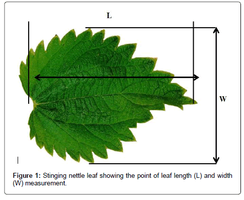
Figure 1: Stinging nettle leaf showing the point of leaf length (L) and width (W) measurement.
In order to determine of fresh weight of leaf (FW), after cutting, samples were weighted on a scale with 0.0001g readability and after drying at 100°C for 24 hr (till constant weight), dry weight of leaves (DW) were determined.
Model building
Three dependent variables (Y) LA, FW and DW were regressed on the independent variables (X) L, W, L+W, L×W, L2, W2, L2+W2 , L2×W2, √(L×W), √L, √W, (L+W)2, FW, DW, (FW)2, (DW)2 , FW×DW, FW+DW, FW2+DW2, √FW, √DW, √(DW×FW) by data from 110 leaves.
In order to select of the best fitted regression models, which represent the relationships between LA, FW and DW as dependent variables and independent variables, after fitting many linear regressions functions, were used the adjusted coefficient of determination (R2), root mean square error (RMSE) and coefficient of variation (CV). The R2, RMSE and CV were three indictors of goodness of fit the models that are calculated by following formula:
 ,
, ,
,
The RMSE of a model prediction is defined as the square root of
Where r is correlation coefficient and r2 is coefficient of determination. Generally for VIF values higher than 10 or T values smaller than 0.10, then collinearity may have more than a trivial impact on the estimates of parameters and consequently one of them should be excluded from the model.
The statistical software SAS 9.1 (SAS Institute Inc, 2011) and Microsoft Excel were used for all computations.
This work examined the relationship between LA, FW and DW as dependent variables and leaf length and width dimensions in an attempt to identify appropriate functions for use in models estimating LA, FW and DW of leaf stinging nettle.
Relationships between LA and different independent variables
Before the model calibration, VIF and T values were calculated to detect collinearity between L and W. The results showed that maximum of VIF and minimum of T were 2.35 and 0.425 respectively. The VIF was less than 10 and T was greater than 0.1 showing that collinearity between L and W can be considered insignificant and negligible [21,22] and L and W can be both included in the model.
Model calibration
Table 1 shows leaf shape parameters as well as various product or sum of L and W that were formulated for prediction of LA individually by linear regression.
| Model No. | Model | Constant ± SE | Reg. coefficient ± SE | RMSE | CV (%) | R2 adjusted |
|---|---|---|---|---|---|---|
| 1 | LA=a+bL | -18.918 ± 2.395 | 4.130 ± 0.219 | 8.62 | 36.86 | 0.76 |
| 2 | LA=a+bW | -19.667± 1.539 | 7.148 ± 0.238 | 5.84 | 24.94 | 0.89 |
| 3 | LA=a+b(L+W) | -24.755 ± 1.461 | 2.959 ± 0.085 | 5.08 | 21.74 | 0.92 |
| 4 | LA=a+b(L×W) | -1.214 ± 0.350 | 0.360 ± 0.004 | 2.13 | 9.12 | 0.98 |
| 5 | LA=a+bL2 | 1.969 ± 1.346 | 0.180 ± 0.009 | 8.32 | 35.00 | 0.78 |
| 6 | LA=a+bW2 | 2.801 ± 0.857 | 0.493 ± 0.016 | 5.67 | 24.23 | 0.89 |
| 7 | LA=a+b(L2+W2) | -0.700 ± 0.811 | 0.15 ± 0.004 | 4.90 | 20.95 | 0.92 |
| 8 | LA=a+b(L2×W2) | 11.928 ± 0.631 | 0.001 ± 0.000 | 5.47 | 23.37 | 0.90 |
| 9 | LA=a+b(√L×W) | -25.014 ± 1.233 | 6.211 ± 0.149 | 4.32 | 18.46 | 0.94 |
| 10 | LA=a+b(L+W)2 | -1.211 ± 0.566 | 0.083 ± 0.001 | 3.42 | 14.63 | 0.96 |
| 11 | LA=a+bFW | 0.800 ± 0.695 | 40.591 ± 0.995 | 4.40 | 18.83 | 0.94 |
| 12 | LA=a+bDW | 2.248 ± 0.839 | 130.260 ± 4.044 | 5.48 | 23.41 | 0.90 |
| 13 | LA=a+b(FW)2 | 12.236 ± 0.705 | 22.876 ± 0.806 | 6.13 | 26.21 | 0.88 |
| 14 | LA=a+b(DW)2 | 14.248 ± 0.927 | 212.613 ± 10.905 | 8.39 | 35.86 | 0.77 |
| 15 | LA=a+b(FW×DW) | 13.015 ± 0.777 | 72.371 ± 2.907 | 6.87 | 29.39 | 0.85 |
| 16 | LA=a+b(FW+DW) | 0.935 ± 0.688 | 31.238 ± 0.760 | 4.37 | 18.70 | 0.94 |
| 17 | LA=a+b(FW2+DW2) | 12.328 ± 0.708 | 20.847 ± 0.741 | 6.18 | 26.41 | 0.88 |
| 18 | LA=a+b(√FW) | -21.022 ± 1.485 | 63.655 ± 1.991 | 5.51 | 23.56 | 0.90 |
| 19 | LA=a+b(√DW) | -19.461 ± 1.621 | 114.060 ± 4.022 | 6.14 | 26.23 | 0.88 |
| 20 | LA=a+b(√FW×DW) | 1.303 ± 0.718 | 73.722 ± 1.895 | 4.60 | 19.68 | 0.93 |
Table 1: The fitted models, constant and regression coefficient with standard error (SE), root mean square error (RMSE), coefficient of variation (CV) and adjusted coefficient of determination (R2) for determination of the best model for leaf area (LA) estimation using length (L), width (W), fresh weight (FW) and dry weight (DW) of leaves measurements.
According to the results, regression analysis showed a strong relationship between LA and some independent variables. Based on selection criteria the best LA estimation model could be identified by comparing models in term of coefficient of determination and RMSE (higher coefficients of determination and lower RMSE and CV).
The highest coefficients of determination 0.98 and 0.96 obtained for LA=a+b(L×W) and LA=a+b(L+W)2 model respectively. Actually 98 and 96% of observed variation for LA could be explained by these models composed of product of leaf L and W and square of sum of leaf L and W. Also these models have the lowest levels of CV 9.12 and 14.63 and RMSE 2.13 and 3.42 respectively. Final developed mathematical model for the best fitted regression model were were LA= -1.21+ 0.36(L×W) and LA=-1.21+0.08(L+W)2. Also the result demonstrated that models based on single variable L or W were more weak compared with two variable models.
Coefficient of determination for LA=a+bFW model indicate that LA estimated by fresh weight as one single measurement is approximately close (94%) to the LA determined by area meter. However models based on L and W measurements offer advantages of non-destructive, easier and require less time for leaf measurements compared with weighing of fresh or dry weight of leaf.
Relationships between FW and DW and different independent variables
The results demonstrated there are strong relationships between FW, DW and some independents variables. Based on selection criteria (previously described) for prediction of FW, the equations that use L×W and (L+W)2 had the highest R2 and lowest RMSE and CV values. Also function consisting LA as independent variable for FW estimation shows a linear strong relationship because of its strong relation with L×W. The equations involving L+W, L2+W2 and √L×W for estimating FW, and L2+W2 for estimating DW showed R2 value higher than 0.91 and RMSE lower than 23.60 (Table 2).
| Model No. | Model | Constant ± SE | Reg. coefficient ± SE | RMSE | CV (%) | R2adjusted |
|---|---|---|---|---|---|---|
| 1 | FW=a+bL | -0.475 ± 0.05 | 0.101 ± 0.00 | 0.191 | 34.25 | 0.80 |
| 2 | FW=a+bW | -0.423 ± 0.05 | 0.163 ± 0.01 | 0.184 | 33.14 | 0.81 |
| 3 | FW=a+b(L+W) | -0.596 ± 0.04 | 0.070 ± 0.00 | 0.129 | 23.18 | 0.91 |
| 4 | FW=a+b(L×W) | -0.018 ± 0.02 | 0.008 ± 0.00 | 0.101 | 18.15 | 0.94 |
| 5 | FW=a+bL2 | 0.035 ± 0.03 | 0.004 ± 0.00 | 0.185 | 33.16 | 0.81 |
| 6 | FW=a+bW2 | 0.095 ± 0.03 | 0.011 ± 0.00 | 0.193 | 34.77 | 0.79 |
| 7 | FW=a+b(L2+W2) | -0.015 ± 0.02 | 0.003 ± 0.00 | 0.12 | 22.19 | 0.91 |
| 8 | FW=a+b(L2×W2) | 0.293 ± 0.02 | 0.004×e-2 ± 0.00 | 0.17 | 30.96 | 0.83 |
| 9 | FW=a+b(√L×W) | -0.583 ± 0.03 | 0.146 ± 0.00 | 0.12 | 22.24 | 0.91 |
| 10 | FW=a+b√ L | -0.475 ± 0.05 | 0.101 ± 0.00 | 0.191 | 34.25 | 0.80 |
| 11 | FW=a+b√W | -0.424 ± 0.05 | 0.163 ± 0.01 | 0.184 | 33.14 | 0.81 |
| 12 | FW=a+b(L+W)2 | -0.023 ± 0.02 | 0.002 ± 0.00 | 0.10 | 18.89 | 0.94 |
| 13 | FW=a+b(LA) | 0.015 ± 0.02 | 0.023 ± 0.00 | 0.10 | 18.89 | 0.94 |
| 1 | DW=a+bL | -0.153 ± 0.01 | 0.031 ± 0.00 | 0.058 | 35.98 | 0.80 |
| 2 | DW=a+bW | -0.122 ± 0.02 | 0.047 ± 0.00 | 0.068 | 41.91 | 0.72 |
| 3 | DW=a+b(L+W) | -0.80 ± 0.01 | 0.021 ± 0.00 | 0.47 | 28.88 | 0.87 |
| 4 | DW=a+b(L×W) | -0.011 ± 0.00 | 0.002 ± 0.00 | 0.037 | 23.08 | 0.92 |
| 5 | DW=a+bL2 | 0.004×e-1 ± 0.00 | 0.001 ± 0.00 | 0.053 | 32.41 | 0.83 |
| 6 | DW=a+bW2 | 0.037 ± 0.01 | 0.003 ± 0.00 | 0.068 | 42.14 | 0.72 |
| 7 | DW=a+b(L2+W2) | -0.012 ± 0.00 | 0.001 ± 0.00 | 0.038 | 23.63 | 0.91 |
| 8 | DW=a+b(L2×W2) | 0.080 ± 0.00 | 0.001×e-2 ± 0.00 | 0.048 | 29.40 | 0.86 |
| 9 | DW=a+b(√L×W) | -0.176 ± 0.01 | 0.043 ± 0.00 | 0.048 | 29.44 | 0.86 |
| 10 | DW=a+b√ L | -0.153 ± 0.02 | 0.031 ± 0.00 | 0.058 | 35.98 | 0.80 |
| 11 | DW=a+b√W | -0.122 ± 0.02 | 0.047 ± 0.00 | 0.068 | 41.91 | 0.72 |
| 12 | DW=a+b(L+W)2 | -0.014 ± 0.00 | 0.006×e-1 ± 0.00 | 0.035 | 21.92 | 0.92 |
| 13 | DW=a+b(LA) | -0.003×e-1 ± 0.01 | 0.007 ± 0.00 | 0.04 | 42.64 | 0.90 |
Table 2: The fitted models, constant and regression coefficient with standard error (SE), root mean square error (RMSE), coefficient of variation (CV) and adjusted coefficient of determination (R2) for determination of the best model for fresh weight (FW) and dry weight (DW) estimation using length (L), width (W), of leaves and leaf area (LA) measurements.
Therefore the best non-destructive proposed linear models for prediction of FW and DW because of simplicity and high accuracy were FW=-0.018+0.008(L×W), FW=-0.023+0.002(L+W)2, DW= -0.011+0.002(L×W) and DW=-0.014+0.006×e-1(L+W)2.
Model validation
In order to validate identified function for prediction of LA, FW and DW, predicted variables LA, FW and DW by the best functions were regressed on measured LA, FW and DW as independent variables (Table 3).
| Model No. | Model | Constant ± SE | Reg. coefficient± SE | RMSE | CV (%) | R2 adjusted |
|---|---|---|---|---|---|---|
| 4 | LA=a+b(L×W) | 0.335 ± 0.335 | 0.986 ± 0.011 | 2.12 | 9.06 | 0.98 |
| 9 | LA=a+b(√L×W) | 1.372 ± 0.663 | 0.941 ± 0.022 | 4.19 | 17.91 | 0.94 |
| 10 | LA=a+b(L+W)2 | 0.861 ± 0.531 | 0.963 ± 0.019 | 3.36 | 14.35 | 0.96 |
| 11 | LA=a+bFW | 1.427 ± 0.675 | 0.939 ± 0.023 | 4.27 | 18.24 | 0.94 |
| 16 | LA=a+b(FW+DW) | 1.408 ± 0.671 | 0.940 ± 0.023 | 4.24 | 18.13 | 0.94 |
| 4 | FW=a+b(L×W) | 0.031 ± 0.005 | 0.944 ± 0.022 | 0.10 | 17.63 | 0.94 |
| 12 | FW=a+b(L+W)2 | 0.034 ± 0.161 | 0.939 ± 0.023 | 0.10 | 18.30 | 0.94 |
| 13 | FW=a+b(LA) | 0.034 ± 0.016 | 0.939 ± 0023 | 0.10 | 18.31 | 0.94 |
| 4 | DW=a+b(L×W) | 0.013 ± 0.005 | 0.917 ± 0.026 | 0.04 | 22.10 | 0.92 |
| 12 | DW=a+b(L+W)2 | 0.012 ± 0.001 | 0.925 ± 0.025 | 0.03 | 21.10 | 0.92 |
Table 3: The constant and regression coefficient with standard error (SE), root mean square error (RMSE), coefficient of variation (CV) and adjusted coefficient of determination (R2) for determination of validation models based on predicted and measured LA, FW and DW.
These linear regressions showed all the proposed relationships, were highly significant (pr<0.0001) with R2 ranged from 0.92 to 0.98. According to t-test the regression lines of measured versus predicted values for LA prediction two models 4 and 10 [L×W and (L+W)2 based] were not significantly different from the 1:1 line correspondence. Slope and intercept for these models were without significant bias from 1 and 0 respectively (pr>0.10). For FW and DW prediction, although models coefficient of determination explained considerable amount of variation except model 4 (based on L×W) for FW and model 12 (based on (L+W)2 for DW, other models slope and constant had significant difference from 1 and 0 at 5% level. This is could be due to high degree of freedom and high power test subsequently.
The results of this study demonstrated the best regression models for prediction of LA=-1.21+ 0.36 (L×W) and LA=-1.21+0.08 (L+W)2 and for FW and DW the suggested linear models are FW=-0.018 + 0.008 (L×W) and DW= -0.014 + 0.0006 (L+W)2. Figure 2 shows scatter plots of observed vs. predicted values of LA, FW and DW using the best and validated models.
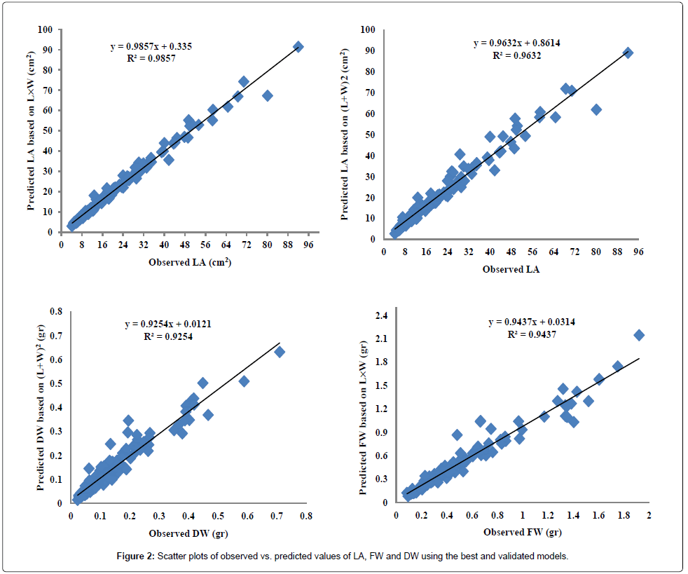
Figure 2: Scatter plots of observed vs. predicted values of LA, FW and DW using the best and validated models.
Stinging nettle (Urtica dioica) herb can be very valuable in the pharmaceutical industry. The most important part of stinging nettle is leaf and leaf area is an important variable in physiological and agronomical researches. As well as plant yield and quality are influenced by photosynthesis and transpiration rate that are intimately linked with leaf area [23]. Therefore recording of leaf area during growth and development can be valuable.
The present study was carried out to develop regression models with high accuracy in prediction of leaf area, fresh weight and dry weight of stinging nettle leaves from simple non-destructive measurements. Twenty models for estimation of leaf area and totally twenty-six models for estimation of leaf fresh and dry weight using different independent variables were tested. Considering all of criteria of selection model in validation including differences between regression coefficient and constant from 1 and 0 respectively, low value for RMSE and CV and high value for R2 adjusted, and model simplicity the best model for LA prediction were based on LA=-1.21+ 0.36(L×W) and LA=- 1.21+0.08(L+W)2 and for prediction of FW and DW, L×W and (L+W)2 based models provided the most accurate estimate. The proposed linear models are FW=-0.018 + 0.008 (L×W) and DW=-0.014 + 0.0006 (L+W)2.
The results of our study in leaf area prediction were consistent with Cristofori et al. [6] who suggested that LA in hazelnut (Corylus avellana L.) and persimmon (Diospyros kaki L.F.) strongly related to L×W. They proposed model LA=2.59 + 0.74 L×W that provided the most accurate (R2 = 0.982)of leaf area in hazelnut and model LA= 3.83 + 0.69 L×W with highest R2=0.98 in persimmon. Similary, Blanco and Folegatti [10] found leaf area of cucumber “Hokushin” could be estimated using the equation based on L×W. They predicted leaf area by model LA=-4.27 + 0.88 L×W with high accuracy and only little differences between the cultivars, location and growing systems. For leaf area prediction models in sugar beet, the results of study of Tsialtas and Maslaris [23] showed model based on both leaf dimensions [LA= 31.928 + 0.5083 L×W] predicted LA better than that using only leaf width or length. Similar reports from Kumar and Sharma [24], Silva et al. [25] and Rouphael et al. [26] in leaf area estimation of clary sage (Salvia sclarea L.), potato (Solanum tubersum L.) and rose (Rosa hybrid L.) respectively.
However, there are several reports those authors [27,28] have used one leaf dimension length or width measurements to predict leaf area. Although models based on one single measurements offer the advantages of more efficient data collection, less complex calculations, and require less time for leaf measurements [29], our finding revealed only length or width were less satisfactory to predict LA, FW and DW in stinging nettle and these models could not confirmed and were eliminated in model validation step.
Confirming the results of previous studies, LA in the stinging nettle could be precisely estimated by measuring leaf dimensions (with calculating L×W) using regression models. Trichomes on the leaves and stems of stinging nettle, injecting several chemicals: acetylcholine, histamine, 5-HT (serotonin), moroidin, leukotrienes, and possibly formic acid that produce stinging sensation when contacted by skin. Therefore for the stinging nettle maybe this is of high importance where easy, non-destructive and especially safe estimation of LA based on simple equation is needed.
Also the results of present study revealed leaf fresh and dry weight could be estimated by dimension product and square of dimension sum using simple function models. However, Chen and Lin [30-32] reported that the linear model could not be used to represent the relationship between dry weights and dimension product and the best predictive equation was based on logarithmic dimension product value. They proposed a power function to predict of leaf dry weight in red hybrid phalaenopsis, grandiflora and multiflora cultivar. Similary, Mokhtarpour et al. [17] showed to predict of leaf fresh and dry weigh in maize, power function gives a better estimation than linear models. But the main advantage of the linear relationships relative to power function is its simplicity of use [23].
According to the results of present study, it can be concluded that leaf area, fresh and dry weight of stinging nettle could be estimated quickly, accurately, non-destructively and safely by using established linear models based on leaf dimensions measurements.