Journal of Pollution Effects & Control
Open Access
ISSN: 2375-4397
ISSN: 2375-4397
Research Article - (2015) Volume 3, Issue 3
The legislation on road traffic noise often requires that acoustic descriptors be determined on a medium or long term. However, such a duration is not feasible for attended monitoring, and therefore, temporal samplings are often applied to save time and resources. However, the values of the noise descriptors estimated by those measured at the sampling times are affected by uncertainty, the amount of which depends on the ratio between the total measurement time and that of the estimate, as well as on the variability of the noise immission at the measurement point.This paper describes the results obtained from the statistical analysis performed on a large set of acoustic data collected at 80 sites along the non-urban road network in the Lombardia region (Italy). The aim of the analysis is to determine the accuracy of two procedures to estimate: i) the daytime (06 to 22 h) A-weighted equivalent level LAeqd and the nighttime (22 to 06 h) A-weighted equivalent level LAeqn from the hourly A-weighted equivalent level LAeqh; and ii) the LAeqh level from the LAeqt measured continuously for a shorter time interval t. The proposed procedures enable to predict the accuracy of both the above estimates; the second one, that is the LAeqh level from the LAeqt, resulted to be greater with increasing of hourly traffic flow and measurement time. Example of the applications of the two procedures is also described.
Keywords: Road traffic noise; Noise monitoring; Temporal sampling; Accuracy
Because road traffic noise is a random phenomenon, the relevant legislation and standards often require the determination of the acoustic descriptors either on a medium or long term. For instance, the day-evening-night level Lden introduced by the European Directive 2002/49/EC (2002) [1], even if referred to 24 h, should be representative of the annual period, and, in Italy, the current legislation requires that the road traffic noise monitoring lasts at least one week [2].
The current instrumentation enables measurements over a long time, as it can store and transmit a large amount of data. However, such duration is not feasible for monitoring attended by an operator and, therefore, requires the time-consuming post processing validation of the acquired data to eliminate all of the sound events that are not associated with road traffic noise. In addition, the need of saving resources and improving the spatial sampling resolution where required often lead to use temporal sampling procedures [3].
These procedures offer the advantage of making the attended monitoring feasible and, therefore, enable to eliminate the data validation. However, the values of the noise descriptors for a medium or long term estimated by those measured at the sampling time are affected by uncertainty, the amount of which depends on the ratio between the measurement time and the medium or long term, as well as on the variability of the noise immission at the measurement point. Several studies on this aspect are available in the literature. For instance, Bordone-Sacerdote et al. [4] described a simple approximate criterion to calculate the uncertainty in evaluating the noise level due to N vehicles per hour, all of the same type, moving with constant speed on one line and direction. Alberola et al. [5] investigated the statistical variability of 2 week’s noise recordings at 50 locations in residential areas affected mainly by road traffic noise. The observed relationships between variability and either logarithmic or arithmetic mean LAeqover the time periods investigated may be of assistance when estimating the noise level variability and the uncertainty associated with a noise measurement affected by road traffic or other environmental noise sources. Theoretical approaches by Makarewicz et al. [6] proposed that the long-term average sound level LAeqT can be approximated by a few, m, short-term, τ, average sound levels, LAeqτ, so that mτ << T, and the uncertainty of such approximation should be calculated by nonlinear uncertainty of ΛΑεθτ for m<10. The analysis of 5 years of continuous noise measurements carried out at one site in Valencia yielded Gaja et al. [7] to conclude that a random day strategy gives a more accurate estimate of the annual equivalent level from the 24-h noise level than a consecutive day’s strategy. Other things being equal, further studies, such as Brambilla et al. [8], confirmed that random sampling is more efficient than continuous one. Bellucci et al. [9] analyzed the noise data collected at 10 sites along non urban roads to evaluate the accuracy of 10 and 20 minute continuous sampling in the estimate of the hourly LAeqh and the day- time (06 ÷ 22 h) LAeqh and night-time (22 ÷ 06 h) LAeqn values. For vehicle passbys during the measurement time greater than 100, the accuracy in the estimate of LAeqh from the measured LAeq was observed to be within ± 1 dB for both the sampling time. Brocolini et al. [10] analyzed acoustic measurements carried out continuously during three months in Paris at six locations, considering samples of 5-min, 10-min, 15-min, 20-min, 30-min and 1-h duration. The results showed that at least 10-min sampling duration is necessary to discriminate among homogeneous time periods.
Predicting the accuracy of the estimated values of LAeq is important because this accuracy can have a large influence on the compliance with the limits required by legislation and standards and the corresponding costs of mitigation actions.
Dealing with the above issue, this paper presents a practical approach for determining and predicting the above accuracy, and the results obtained from the statistical analysis performed on a large set of acoustic data collected from continuous monitoring during weekdays in 80 sites alongside the non-urban road network in the Lombardia region (Italy) are described. The roads have different layouts: from the widest two carriage ways with three lanes for each direction to the narrowest one carriageway with one lane for each direction.
The aim of the analysis has been twofold, that is to determine the accuracy of:
• the estimate of daytime (06 to 22 h) A-weighted equivalent level LAeqd and nighttime (22 to 06 h) A-weighted equivalent level LAeqn from the 24-hr hourly pattern of A-weighted equivalent level LAeqh;
• the estimate of hourly LAeqh from LAeqt measured continuously for different shorter durations, namely t=5, 10, 15, 20 and 30 minutes.
The analysis was performed considering the hourly traffic flow too.
The acoustic monitoring carried out on weekdays in the 80 sites alongside the network of non-urban roads in the Lombardia region in the years 2000-2006 has provided a large database containing not only the A-weighted equivalent level LAeq measured at a sampling rate of 1 minute (LAeq1m) but also, at 15 sites, the hourly traffic flow for 24 hours. At another 35 sites the traffic flow was available for 1 hour during the daytime. The traffic was always free flowing during the monitoring and the microphone was located at 3 up to 60 m from kerbside, as already described in Zambon et al. [11].
The LAeq1m data have been pooled to obtain the corresponding values LAeqt at the times t of 5, 10, 15, 20, 30 and 60 minutes, as well as the daytime LAeqd and nighttime LAeqn levels.
The ranges of the daytime LAeqd and nighttime LAeqn in the 80 sites were very wide, as reported in Table 1, and the distributions of the hourly LAeqh levels, with a bin width of 1.5 dB, are shown in Figure 1. The difference between the mean values of day and night LAeqh distributions was 7.0 dB. (Table 1) (Figure 1).
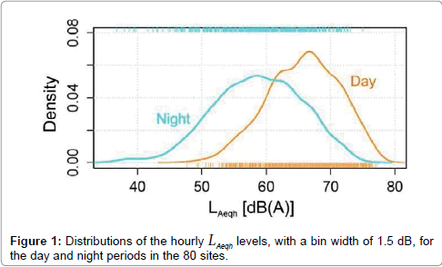
Figure 1: Distributions of the hourly LAeqh levels, with a bin width of 1.5 dB, for the day and night periods in the 80 sites.
| LAeq [dB] | Max | Min | Range |
| LAeqd (06-22 h) | 76.3 | 51.7 | 24.6 |
| LAeqn (22-06 h) | 71.4 | 52.6 | 18.8 |
Table 1: Ranges of daytime LAeqd and nighttime LAeqn in the 80 sites.
At the 21 sites where the monitoring was performed for longer than 24 hr the median of the corresponding LAeqh values for each ith hour was considered. This led to 59 (80-21) profiles of hourly LAeqh available for the statistical analysis. The median was preferred to the mean value because the former is less influenced by outliers. This data pooling avoided that 24-h LAeqh profiles measured at the same road but on different days could be allocated to different groups by the subsequent cluster analysis.
Because the measurements were performed in various environmental setups, a direct comparison among the 24-h profiles of the hourly LAeqh was not meaningful. For this reason, and to perform further statistical analysis of the data, each ith value of hourly LAeqh in the jth temporal series was referred to the corresponding daytime level, LAeqdj, and the difference δij was considered:
δij=LAeqhij-LAeqdj[dB](i=1, ……., 24; j=1, ……., 59) (1)
as shown in the example in Figure 2.
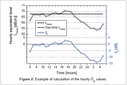
Figure 2: Example of calculation of the hourly dij values.
The reference to the daytime LAeqd was chosen because this descriptor is more often available than the night time LAeqn. However, the methodology of the procedures described in the following for the estimate of daytime LAeqd can be also applied to develop similar procedures for estimating the nighttime LAeqn, providing that each ith value of hourly LAeqh in the jth temporal series is referred to the corresponding nighttime level, LAeqnj. Table 2 reports the distribution of the 24-h profiles of the hourly LAeqh available for the statistical analysis.
| Day | Mo | Tu | We | Th | Fr | Total |
| N. profiles j | 14 | 26 | 19 | 26 | 23 | 108 |
Table 2: Distribution among the weekdays of the 24-h profiles jth of the hourly LAeqh.
The 24-h profiles were grouped according to the day of monitoring (Monday to Friday). In addition, the unsupervised technique of clustering was used to group together profiles which are “close” to one another in a multidimensional feature space, to uncover some inherent structure of the data. Various clustering algorithms were used, namely the hierarchicalagglomeration using the Ward method [12], the K-means using the Hartigan and Wong algorithm [13], the partitioning around medoids by Kaufman and Rousseeuw [14] and the model-based method. The results of these algorithms were compared and the most appropriate number of clusters for the data, a compromise between satisfactory discrimination and the need of limited number of clusters, was chosen. The range of solutions for clustering k was set from five groups (for a straightforward comparison with the categorization according to the day of monitoring) to two groups, which corresponds with the minimal discrimination. The Euclidean distance was chosen as the metric of the distance among observations.
The statistical software R (an open-source programming environment for data analysis, graphics and statistical computing) was applied for the above clustering and the package “clValid” by Brock et al. [15-17] was used to validate the results. For such validation, three features of the cluster partitions were considered, namely, compactness, connectedness, and separation. Connectedness relates to the extent to which observations are placed in the same cluster and is measured by the connectivity [18]. The connectivity has a value between zero and ∞ and should be minimized. Compactness assesses cluster homogeneity, usually by examining the intra-cluster variance, while separation quantifies the degree of separation between clusters (usually by measuring the distance between cluster centroids). Because compactness and separation demonstrate opposing trends (compactness increases with the number of clusters but separation decreases), popular methods combine the two measures into a single score, such as the Dunn index [19] and silhouette width [20]. The Dunn index has a value between zero and ∞ and should be maximized. The silhouette width lies in the interval (-1, 1) and should be maximized.
Considering the estimate of the hourly LAeqh from the LAeqt level measured continuously for a shorter time t:
t=m·M [s]with 0 < m < 1 (2)
where M=3600 s, the LAeqt values referring to the measurement times t of 5, 10, 15, 20 and 30 minutes were compared with the corresponding hourly LAeqh to determine the difference:
ετ=LAeqt - LAeqh [dB] (3)
Thus, with the assumption that the estimated LAeqh is equal to the measured LAeqt, the above difference represents the error εt of such estimate. The errors ετ were analyzed as function of the standard deviation of the LAeqt belonging to the relevant hour and the hourly traffic flow, as well as in terms of the probability PtE that the accuracy of the hourly LAeqh estimate from LAeqt is within a specific interval E, namely ± 0.5 and ± 1.0 dB with an interval width of 1 and 2 dB respectively. The value of probability PtE was obtained by the number of measurements within the selected interval divided by the total number of measurements.
The available data sets for the above analyses are reported in Table 3.
| N. of samples | Measurement time t [minute] | ||||
| 5 | 10 | 15 | 20 | 30 | |
| No traffic flow data | 7056 | 3528 | 2352 | 1764 | 1176 |
| Traffic flow data | 28176 | 14088 | 9392 | 7044 | 4696 |
| Total | 35232 | 17616 | 11744 | 8808 | 5872 |
Table 3: Data sets available to determine the difference εt = LAeqt - LAeqh.
The main results of the estimate of the daytime LAeqd from the hourly LAeqh and those of the estimate of the hourly LAeqh from the LAeqt values measured continuously for shorter time t are described separately.
Estimate of daytime LAeqd from the hourly LAeqh
Figure 3 shows the 24-h profiles of the average δij for each weekday from Monday to Friday. By this data grouping overlaps of the profiles occur very often, especially during the day period from 06 to 22 h. For the night period (22 to 06 h) the highest and lowest average profiles correspond to Friday and Monday, respectively.
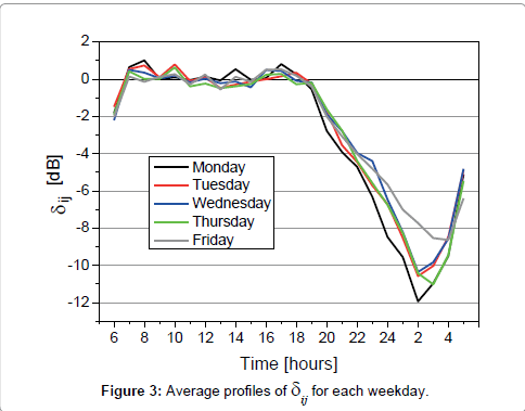
Figure 3: Average profiles of dij for each weekday.
A different classification was obtained by clustering. Table 4 summarizes the output of the validation of the results obtained by the various clustering methods in terms of the optimal scores observed for the connectivity, the Dunn index and the silhouette width.
| Feature | Value | Method | No. of clusters k |
| Connectivity | 17.85 | PAM | 2 |
| Dunn index | 0.17 | Model | 3 |
| Silhouette width | 0.26 | K-means | 2 |
Table 4: Optimal scores obtained by the “clValid” package for the cluster validation.
After the analysis of the detailed results for each clustering method, the two groups obtained by the K-means were considered to be a reasonable solution, also because the corresponding values of the Dunn index and the connectivity were not too much different from the optimal scores (0.13 and 18.55 respectively). Figure 4 shows the results of the multidimensional scaling (MDS) applied to the data to provide a visual representation of the pattern of proximities among the data.
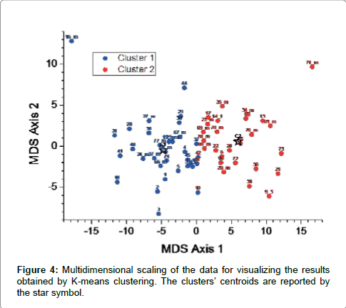
Figure 4: Multidimensional scaling of the data for visualizing the results obtained by K-means clustering. The clusters’ centroids are reported by the star symbol.
The discrimination between the two clusters is rather good; the centroids C1 and C2 are reported by stars in the plot. Cluster 1 and 2 are formed by 33 and 26 profiles respectively and their correspondence (in percentage) with the categorization based on weekdays is reported in Table 5. For each day the 24-h profiles are not too much unevenly splitted into the two clusters. Cluster 2 groups the majority of profiles observed on Monday, whereas Cluster 1 is formed by the majority of profiles of the other weekdays.
| Cluster membership | Mo | Tu | We | Th | Fr |
| 1 | 40.0 | 56.7 | 58.8 | 51.8 | 61.9 |
| 2 | 60.0 | 43.3 | 41.2 | 48.2 | 38.1 |
Table 5: Distribution (%) of 24-h profiles of δij in each cluster considering the day of monitoring.
The average profiles δik for each cluster and the standard error of the mean at 95% confidence interval are shown in Figure 5. Because the distributions of data were not normal for some hours, the mean and its confidence intervals were calculated using the bootstrap method [21] considering 1000 samples with replication.
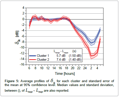
Figure 5: Average profiles of dik for each cluster and standard error of the mean at 95% confidence level. Median values and standard deviation, between (), of LAeqd – LAeqn are also reported.
The hourly intervals with significant differences between the two average profiles at the confidence level of 95% were identified by the Mann-Whitney test and are listed in Table 6 with the corresponding significance value. The best discrimination between the clusters occurs during the nighttime (22-06 h). In the 07-19 h period, the average profile of cluster 1 has very small fluctuations around the LAeqd, whereas that of cluster 2 shows larger fluctuations, but still within 1 dB. The median value of the difference LAeqd – LAeqn, together with the standard deviation value given within ( ), is also reported in Figure 5: cluster 1 show a value 1.7 dB lower than that observed for cluster 2. As the noise emission of the road under consideration is not known “a priori”, additional information linked to such emission, i.e. traffic flow is necessary for the selection of the average profile most appropriate for the road itself. For this purpose, the average daily traffic flows (ADT) and their 95% confidence intervals for all the roads belonging to each cluster were calculated by the bootstrap method. The results are reported in Table 7.
| Hourly interval | Significance 95% | Hourly interval | Significance 95% |
| 6-7 | 0.003 | 23-24 | 0.000 |
| 7-8 | 0.029 | 0-1 | 0.000 |
| 8-9 | 0.026 | 1-2 | 0.000 |
| 11-12 | 0.028 | 2-3 | 0.000 |
| 15-16 | 0.008 | 3-4 | 0.000 |
| 21-22 | 0.015 | 4-5 | 0.000 |
| 22-23 | 0.000 | 5-6 | 0.000 |
Table 6: Hourly intervals of the average profiles of the two clusters with significant differences at the confidence level of 95%.
| Average daily traffic flow ADT [vehicles] | Cluster | 1 | 2 |
| Mean | 25223 | 17470 | |
| + 95% C.I. | 31084 | 20412 | |
| - 95% C.I | 20755 | 14588 |
Table 7: Average daily traffic flow of the roads according to their cluster membership.
The boxplot of the ADT values given in Figure 6 shows a clear overlap of the data associated to the two clusters which leads to uncertainty in the selection of the appropriate profile. Thus, this parameter is not suitable for the above purpose. To overcome this problem a deeper analysis of traffic flows was performed on hourly basis. The Mann-Whitney test, which was applied to the hourly traffic flows of the roads according to their cluster membership, showed that the differences among means were not different at the 95% confidence level for the period between 10 and 16 h, as shown in Figure 7, where the hourly average values of traffic flow and the corresponding 95% confidence interval are reported.
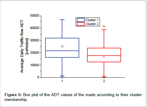
Figure 6: Box plot of the ADT values of the roads according to their cluster membership.
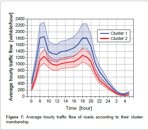
Figure 7: Average hourly traffic flow of roads according to their cluster membership.
Thus, the hourly traffic flow is suitable for the appropriate selection of the cluster average profile, providing that it is not measured in the 10-16 h period. After all, traffic flow data are usually available for rush hours, which usually are outside the overlapping period, as shown in Figure 7. Cluster 1 includes the busiest roads. On the other hand, looking at the hourly cluster profiles and their corresponding 95% confidence intervals plotted in Figure 5, and zoomed in for the day period 7-19 h in Figure 8, the hourly intervals most suitable for the best accuracy in the LAeqd estimate are observed in the period from 12 to 16 h for both clusters.
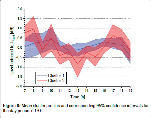
Figure 8: Mean cluster profiles and corresponding 95% confidence intervals for the day period 7-19 h.
Estimate of hourly LAeqh from LAeqt measured for shorter time interval t
The hourly LAeqh is not often measured continuously, whereas it is frequently estimated by the LAeqt values measured for a shorter time t according to the following relationship:
 (4)
(4)
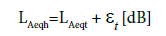
To evaluate the accuracy ετ of such an estimate, the differences εt in equation (3), calculated for the measurement times t of 5, 10, 15, 20 and 30 minutes, were determined for all the monitoring data considering their cluster memberships. Figure 9 shows the box plots of the obtained values of εt for each measurement time t and cluster.
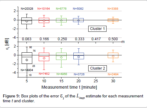
Figure 9: Box plots of the error et of the LAeqh estimate for each measurement time t and cluster.
As expected, the amplitude of the error εt decreases with the increase of the measurement time t and the means and median tend to the null value. For each measurement time t, the mean closest to zero and smallest standard deviation are observed for cluster 1 which includes roads with the highest traffic flows. The Kolmogorov-Smirnov test showed that all the distributions were not normal at 95% significance level, with means and standard deviations reported in Table 8.
| Cluster | Measurement time t [minute] | |||||
| 5 | 10 | 15 | 20 | 30 | ||
| 1 |  |
-0.29 | -0.16 | -0.11 | -0.08 | -0.05 |
| s | 1.79 | 1.32 | 1.11 | 0.99 | 0.82 | |
| 2 |  |
-1.08 | -0.68 | -0.50 | -0.38 | -0.23 |
| s | 3.61 | 2.80 | 2.38 | 2.10 | 1.67 | |
Table 8: Means  and standard deviations s of the error εt [dB] for each measurement time t and cluster.
In order to predict the error εt for each measurement time, the median absolute value of the error  of the LAeqh estimate obtained from LAeqt was related to the hourly traffic flow. The traffic flow data were grouped in bins with a width of 100 vehicles/hour, and the median absolute value of the error in each bin was considered. The plots in Figure 10 report the traffic flow on the x axis on a log scale and show the regression lines for the five t measurement times and the two clusters. For a fixed hourly traffic flow, the errors observed for cluster 2 are greater than those for cluster 1 and, as expected, for both clusters the errors decrease with increasing of traffic flow and measurement time t. In addition, for a fixed measurement time t the regression line for cluster 2 is steeper than that for cluster 1.
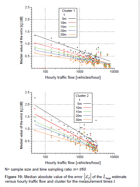
Figure 10: Median absolute value of the error of the LAeqh estimate versus hourly traffic flow and cluster for the measurement times t.
Table 9 reports the values of parameters A and B in the relationship used for the data interpolation, together with the adjusted Pearson’s correlation coefficient R2. The last column gives the parameters obtained by interpolation of all the data, regardless their cluster membership.
| y = A + B . log(x) | Cluster | All data | ||
| t [min] | Coefficient | 1 | 2 | |
| 5 | A | 2.20 | 3.43 | 2.73 |
| B | -0.49 | -0.86 | -0.66 | |
| Adj. R2 | 0.29 | 0.69 | 0.85 | |
| 10 | A | 1.72 | 2.87 | 2.08 |
| B | -0.39 | -0.74 | -0.50 | |
| Adj. R2 | 0.68 | 0.81 | 0.79 | |
| 15 | A | 1.37 | 2.31 | 1.65 |
| B | -0.30 | -0.59 | -0.38 | |
| Adj. R2 | 0.47 | 0.74 | 0.62 | |
| 20 | A | 1.19 | 2.13 | 1.48 |
| B | -0.26 | -0.55 | -0.35 | |
| Adj. R2 | 0.50 | 0.79 | 0.64 | |
| 30 | A | 0.99 | 1.65 | 1.20 |
| B | -0.22 | -0.42 | -0.28 | |
| Adj. R2 | 0.39 | 0.64 | 0.55 | |
Figure 9: Values of A and B parameters in the relationship used for the data interpolation of median  and hourly traffic flow (x).
The differences in the accuracy of the LAeqh estimate obtained by the sampling times decrease with the increasing of the hourly traffic flow, as clearly shown in Figure 11 for all the data pooled together. The 30 minute sampling was taken as reference as it was the most accurate in the LAeqh estimate and the y axis reports the corresponding differences of the median absolute value of the error  for the sampling times t=5, 10, 15 and 20 minutes; greater this difference lower the accuracy. It can be seen that above 4000 vehicles/hour the 10 minute sampling performs slightly better than the 15 minute one, but the former is more dependent on the traffic flow rather than the latter (slope of the regression line steeper).
Figure 11: Differences  of the median absolute value of the error for the sampling times t= 5, 10, 15 and 20 minutes referred to the 30 minute sampling regardless the cluster membership.
The results for the measurement time t=10 minutes were compared with those obtained in a previous similar study carried out along nonurban roads in the Lazio region in Italy [9]. As can be seen in Figure 12, the regression relationship of the data collected in the Lazio region is steeper than that obtained for the present study, but the differences are rather small and increase with increasing of hourly traffic flow.
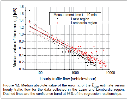
Figure 12: Median absolute value of the error  of the LAeqh estimate versus hourly traffic flow for the data collected in the Lazio and Lombardia region. Dashed lines are the confidence band at 95% of the regression relationships.
Dealing with the probability PtE that ετ is within a specific accuracy range, Figure 13 reports the regression lines obtained by fitting the data of the hourly traffic flow with those corresponding to the five measurement times for the accuracy range of ± 0.5 dB and for both the clusters. The values of regression parameters obtained from fitting are given in Table 10, together with the adjusted Pearson’s correlation coefficient R2. The last column gives the parameters obtained by interpolation of all the data, regardless their cluster membership. The probabilities Pt0.5 obtained for cluster 2 are lower than those for cluster 1 and these differences decrease with increasing of hourly traffic flow.
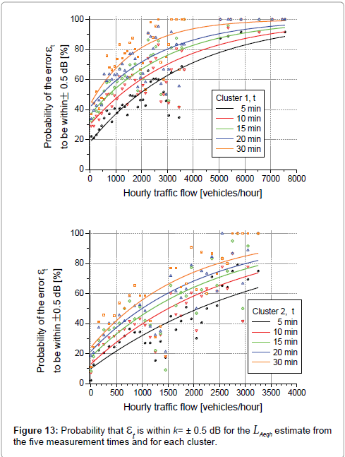
Figure 13: Probability that et is within k= ± 0.5 dB for the LAeqh estimate from the five measurement times and for each cluster.
| y = 100-(A.Bx) | Cluster | All data | ||
| t [min] | Coefficient | 1 | 2 | |
| 5 | A | 81.91 | 89.99 | 85.93 |
| B | 0.99974 | 0.99972 | 0.99973 | |
| Adj. R2 | 0.81 | 0.69 | 0.82 | |
| 10 | A | 70.07 | 86.91 | 77.27 |
| B | 0.99972 | 0.99963 | 0.99969 | |
| Adj. R2 | 0.72 | 0.63 | 0.79 | |
| 15 | A | 63.63 | 82.18 | 71.86 |
| B | 0.99967 | 0.99959 | 0.99965 | |
| Adj. R2 | 0.65 | 0.59 | 0.71 | |
| 20 | A | 58.67 | 78.46 | 66.34 |
| B | 0.99964 | 0.99955 | 0.99963 | |
| Adj. R2 | 0.66 | 0.65 | 0.68 | |
| 30 | A | 56.81 | 75.77 | 65.59 |
| B | 0.99945 | 0.99946 | 0.99947 | |
| Adj. R2 | 0.66 | 0.62 | 0.68 | |
Table 10: Values of regression parameters obtained from the εt data fitting as a function of hourly traffic flow and for the accuracy range E = ± 0.5 dB (x is the hourly traffic flow).
The above mentioned probabilities Pt0.5 were compared with those computed according to the following relationship proposed by Bordone-Sacerdote et al. [4]:
 (5)
(5)
where T=3600 s, t is the measurement time [s], N the hourly traffic flow, n the vehicles counted in the measurement time t calculated by:
 (6)
(6)
n1 and n2 the uncertainty in vehicle counting corresponding to the uncertainty E=± 0.5 dB in the noise level, that is:
 (7)
(7)
 (8)
(8)
Equation 5 provides values Pt0.5 with the assumption of N vehicles per hour, all of the same type, moving with constant speed on one line and direction. Figure 14 shows that the experimental data and their fitting (solid lines) are rather lower than the corresponding values provided by equation (5), reported by dashed lines. This is most likely due to the difference between real traffic conditions and those assumed for equation (5).
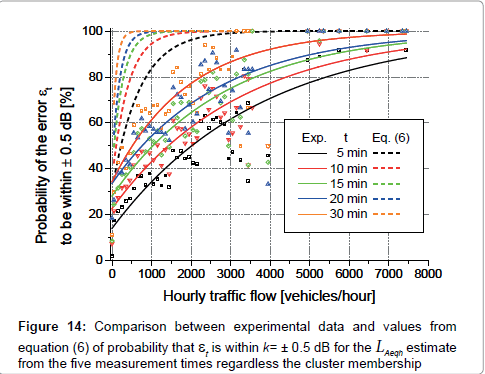
Figure 14: Comparison between experimental data and values from equation (6) of probability that et is within k= ± 0.5 dB for the LAeqh estimate from the five measurement times regardless the cluster membership
Regarding the accuracy range of E= ± 1.0 dB, as expected higher probability Pt1.0, other factors being equal, were observed as shown in Figure 15, dealing with all the data, regardless their cluster membership. For instance, for t=15 minute at the hourly traffic flow of 1000 vehicles/ hour, widening the accuracy range from ± 0.5 to ± 1.0 dB increases the probability P15mE by 26.1% (from 49.4 at ± 0.5 dB up to 75.5% at ± 1.0 dB).
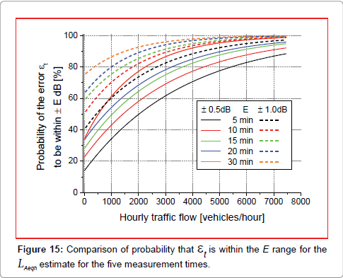
Figure 15: Comparison of probability that et is within the E range for the LAeqh estimate for the five measurement times.
Example of application
To illustrate the features of the procedures above described and the associated uncertainties in the estimation, let assume that the road traffic monitoring carried out continuously for 15 minutes in the interval 8:15-8:30 h gives LAeq15=64.0 dB(A) and traffic flow=250 vehicles during the 15 min measurement time. Assuming that the traffic flow is evenly distributed throughout the hourly interval from 8 to 9 h, the corresponding hourly traffic flow is 250×4=1000 vehicles/hour. Thus, the road can be associated with cluster 2 (see Figure 7) and for the 15 min measurement time, the median value of ![]() is estimated to be as shown in Figure 10 and Table 9
is estimated to be as shown in Figure 10 and Table 9
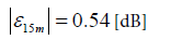 (9)
(9)
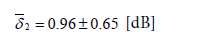
which can be assumed as standard uncertainty of the estimate of the hourly LAeqh from the measured LAeq15m for 15 minutes. For the 8-9 hourly intervals and cluster 2, Figure 8 provides the corresponding δη value:
 (10)
(10)
Thus, the estimated value of the day LAeqd is equal to:
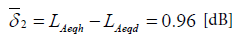 (11)
(11)
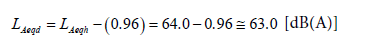 (12)
(12)
With standard uncertainty of 0.65 dB. The combined uncertainty of the two procedures, under the simplifying hypothesis that they are uncorrelated, is calculated by:
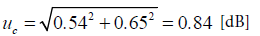 (13)
(13)
Considering the coverage factor k=1.96 corresponding to the 95% confidence level, the estimated daytime LAeqd with the expanded uncertainty is as follows:
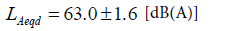 (14)
(14)
Considering the estimate of LAeqn, in addition to the similar procedures which can be developed as described for LAeqd estimate, a straightforward calculation can be based on the estimated value of LAeqd, considering the median value of the differences LAeqd – LAeqn and taking as standard uncertainty of such estimate the standard deviation of these differences. Thus, Figure 5 shows for cluster 2 the median value and standard deviation s as follows:
 (15)
(15)
 (16)
(16)
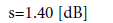
Then:
 (17)
(17)
with a standard uncertainty of 1.4 dB.
However, the above uncertainty budgets are limited to the proposed procedures under the simplified hypothesis that these are uncorrelated; the standard uncertainties due to the other sources, at least that due to the instrumentation, should be considered, for instance as described by Craven et al. [22].