The spotted seatrout (Cynoscion nebulosus Cuvier) is the most popular recreational marine finfish in Texas [1] and is common throughout the Gulf of Mexico (hereafter Gulf). As such, the Texas Parks and Wildlife Department manage this species intensively, and management includes annual large-scale stock enhancement in four Texas bays (Lower Laguna Madre, Upper Laguna Madre, Galveston Bay and Sabine Lake). Because of the direct and intensive management of this species, it is imperative that management goals account for the possibility of discreet subpopulations (genetic structure) within Texas waters. Previous genetic examinations of population structure of spotted seatrout in the northern Gulf, and along the Texas coast in particular, have resulted in two general models of spotted seatrout genetic structure within the Gulf.

Weinstein and Yerger [2] used allozyme data to characterize genetic diversity in spotted seatrout from the Gulf coast of Florida, and concluded that spotted seatrout were organized into discreet subpopulations. Gold et al. [3] used the distribution of mitochondrial DNA (mtDNA) RFLP haplotypes to conclude that samples taken of spotted seatrout throughout the northern Gulf and Atlantic (including samples from Texas) generally represented distinct subpopulations, and suggested that these subpopulations may be organized by natal estuaries, as expected from short dispersal distances in tagging studies and the affinity of spotted seatrout for inshore areas. In contrast with the finding of discreet subpopulations, Ramsey and Wakeman [4] and King and Pate [5] used allozymes and found low measures of population subdivision (F_st) and high gene flow (N_em) in Gulf samples, indicating that individuals in the western/northern Gulf comprise a single large population. Both studies found isolation-by-distance (IBD) among locales, suggesting that genetic differentiation occurred on a broad (but continuous) geographic scale. Recently, the authors of this study examined mtDNA control region haplotype data and reached a similar conclusion of IBD; evidence for discreet subpopulations was weak, and driven primarily by divergence at the extreme ends of the sampling distribution [6]. In any event, the effective genetic differences between distinctive subpopulations, versus a single population operating under IBD, are likely to be subtle because the genetic drift that is expected among distinctive subpopulations can potentially be offset by the large census sizes that generally characterize marine finfish populations. Thus, Gold et al. [7] suggested that although subpopulations centered in natal estuaries may have distinctive short-term demographic characteristics, recurrent gene flow among adjacent estuaries results in a genetic pattern which resembles IBD, rather than distinct subpopulations.

In all previous studies, an empirical method for formulating hypotheses regarding the geographic size and demography of putative spotted seatrout subpopulations has not yet been employed. These studies have generally invoked the assumption that subpopulations will most likely be geographically centered within inshore bays and estuaries. However, Anderson and Karel [6] pointed out that there was little physical structure available that could act as barriers to limit migration among most inshore areas in Texas. Thus, the spatial component of designated estuaries along the coast of Texas amount to little more than political designations, rather than disparate entities with completely independent geography. In this study, a novel approach to defining putative subpopulation boundaries was used to develop hypotheses regarding the genetic structure of spotted seatrout in Texas. A geospatial data set representing the abundance of spotted seatrout in Texas’ inshore coastal areas was extracted from a fishery-independent database of 33 years of Texas Parks and Wildlife Department gill net sampling. These data were used to construct a map of spotted seatrout abundance along the entire Texas coast, which resulted in a more systematic basis upon which putative subpopulation boundaries could be formulated. That is, subpopulation boundaries might be expected to occur in areas where spotted seatrout abundance was relatively low. These putative boundaries were then evaluated quantitatively by genetic data analysis. Two genetic data sets were examined: 1) the mtDNA sequence data of Anderson and Karel [6] was reanalyzed, and 2) a new data set of microsatellite markers was added. The results of the current study were evaluated in the context of all other previous studies [2-8], and were used to add resolution to the question of population structure of spotted seatrout on the coast of Texas.

Gill net sampling and geospatial data

Spatial data was generated by collating standardized gill net catch data from 1.85 km-square shoreline grids covering the extent of the Texas coast. Gill nets have been deployed biannually coast-wide for 33 years, during fishery-independent departmental monitoring by the Texas Parks and Wildlife Coastal Fisheries Division (hereafter TPWD). Each major estuarine system has been sampled weekly, for a 10 week period during the spring and a 10 week period during the fall. Grids for sampling are chosen at random with 3-5 grids sampled per week, and no grid is sampled twice in the same month. Gill nets, with mesh sizes ranging from 76 mm to 152 mm, were 184 m long and partitioned into four 46 m sections. This data set comprised 22,824 data points covering the extent of the Texas shoreline for years 1975-2008, including the bay side of barrier islands and peninsulas.

For each grid, catch-per-unit-effort (CPUE) was assessed by averaging multiple independent records of CPUE over time. Averaged CPUE was then rounded to the nearest whole integer, and each grid was categorized as having a CPUE of 0, 1, 2 or 3+ over the entire sampling period. Category scores were then superimposed as abundance-graded circles over grids on the Texas shoreline using ArcMap v9.3 (ESRI, Redlands, CA, USA). The abundance data was examined (qualitatively) for areas where multiple adjacent grids had low average abundance (CPUE = 0). These areas were hypothesized to be putative subpopulation boundaries, which were evaluated quantitatively using genetic methods (see below).

Mitochondrial DNA sequence data

The data set of Anderson and Karel [6] was reanalyzed here to examine patterns of mtDNA control region haplotype distribution which correlated with geospatial data. Briefly, this data set comprised young-of-the-year (YOY) spotted seatrout from eight of Texas’ nine major bay systems over a three year period (hereafter, SL = Sabine Lake; EM = East Matagorda Bay; WM = West Matagorda Bay; SB = San Antonio Bay; AB = Aransas Bay; CC = Corpus Christi Bay; UL = Upper Laguna Madre; LL = Lower Laguna Madre, Fig. 1). Within each bay, care was taken to avoid sampling possible family groups, by taking individuals from multiple sampling locales on multiple dates. Samples consisted of either >200 mg fin clips, or whole fish in the case of small individuals. Samples were preserved and processed according to Anderson and Karel [6].

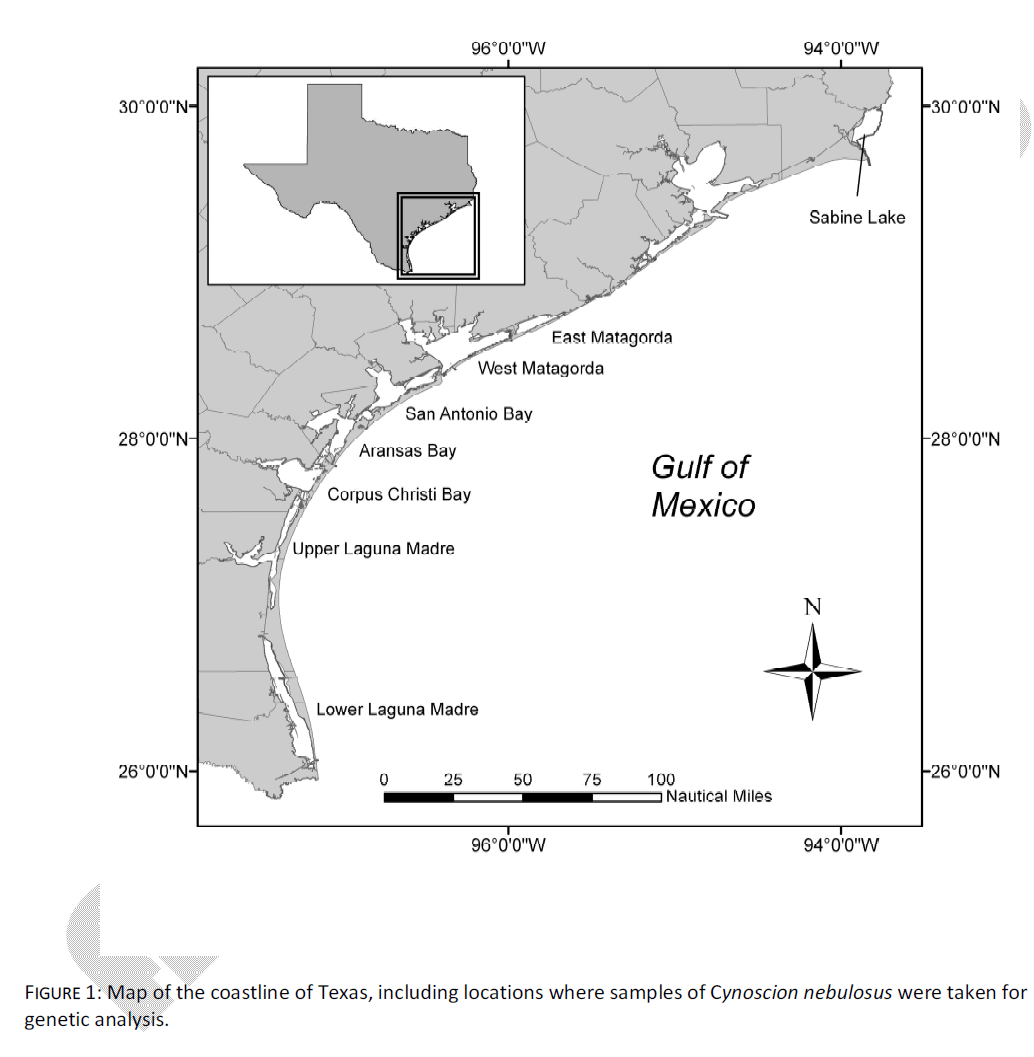
Figure 1: Map of the coastline of Texas, including locations where samples of Cynoscion nebulosus were taken for genetic analysis.

Genetic differentiation among groups and among samples (localities) within groups was tested with an analysis of molecular variance (AMOVA, [9]). Individual samples were pooled across years and variance in mtDNA haplotype association was partitioned into between-individual, among-samples and among-group effects using ARLEQUIN v3.0 [10], using simple pair wise differences. Four different models of population structure were tested, as follows: 1) all sampling locales grouped as single subpopulations (SL) + (EM) + (WM) + (SB) + (AB) + (CC) + (UL) + (LL), 2) three subpopulations consisting of (SL) + (EM, WM, SB, AB, CC) + (UL, LL), 3) three subpopulations consisting of (SL) + (EM, WM, SB, AB, CC, UL) + (LL), and 4) four subpopulations consisting of (SL) + (EM, WM, SB, AB, CC) + (UL) + (LL). These models were chosen based on the low abundance of spotted seatrout in areas between LL and UL, between UL and CC, and between EM and SL, as indicated from examination of the geospatial data set (see results). A Mantel matrix correlation analysis was also used to examine isolation-by-distance effects. This Mantel procedure was identical to that of Anderson and Karel [6] and is only presented here for comparison purposes to a similar Mantel matrix test on the microsatellite data.

Finally, a hierarchical cluster analysis was performed on pairwise DNA distance data between samples, in order to determine the number of groups (subpopulations) present in the data set, and to simultaneously determine group membership. Nei’s corrected genetic distance [11] was generated between each pair wise set of samples. The dissimilarity matrix of Nei’s values was then subjected to clustering using Ward’s minimum variance linkage method [12]. This method was chosen because it minimizes within-group dispersion and is effective in eliciting among-cluster relationships [13], which is preferred in situations where clusters are expected to be defined by short distance. The number of clusters to retain was determined qualitatively by using an elbow-plot of genetic distance values; that is, the expected group number was equal to the number of clusters (k) present as the genetic distance accounted for by each successive addition of clusters leveled off. Thus, within-group dispersion minimization was not improved with additional levels of clustering, once the optimum number of clusters had been obtained. Clustering was conducted using JMP 7.0.1 software (SAS Institute, Cary, NC, USA). Statistical support for major nodes on the cluster dendrogram was obtained by bootstrap analysis using PHYLIP 3.63 software [14], with 100 bootstrap replications over geographic samples.

Microsatellite marker data

For the microsatellite data set, spotted seatrout YOY were collected over a three-year period from the same eight geographic localities as those from the mtDNA data set. In some, but not all cases, samples from the mtDNA and microsatellite data sets overlapped. Each data set was collected and analyzed at different times; although congruence in samples used was attempted, in some cases samples were no longer available or were degraded. For this reason, each data set will be treated independently. Microsatellite samples were taken as either whole fish or as fin clips of larger fish and submerged immediately in vials containing 95% ethanol (EtOH). The vials were placed on ice or stored at 4ºC for 24 hours prior to shipment to the Perry R. Bass Marine Fisheries Research Station (PRBMFRS).

Once at PRBMFRS, samples were stored in ethanol at room temperature for an indeterminate period. Approximately 200 mg of tissue were used for individual DNA isolations. All DNA isolations were carried out using PUREGENE® DNA isolation kits (Gentra Systems, Inc., Minneapolis, MN), with a final rehydration volume of 75 μl.

Six microsatellite loci were used to examine population structure in spotted seatrout (Table 1). These loci were developed from the closely related Sciaenid Sciaenops ocellatus, and initial characterization of these loci can be found elsewhere [15,16]. These loci were amplified via the Polymerase Chain Reaction (PCR) under a modified touchdown protocol, using Ready-To-Go™ PCR beads (GE Healthcare, Piscataway, New Jersey) on a Techne Genius thermocycler (Techne Inc., Princeton, New Jersey). Reactions consisted of 1 μl template DNA (50 ng/μl), 1 Ready-To-Go™ bead, and 24 μl of forward and reverse primer cocktail (0.4 μM standard primer concentration of each primer), for a total of 25 μl. Each reverse primer oligonucleotide was purchased labeled with a WellRED dye (Sigma-Proligo, Boulder, Colorado) in preparation for visualizing on a Beckman-Coulter CEQ8000_™ automated sequencer (Beckman Coulter Inc., Fullerton, California). The touchdown PCR protocol utilized for all reactions consisted of the following: an initial single denature period of 2 min at 95oC, 10 cycles of initial amplification (95oC for 30 s, 55oC for 30 s lowering 1oC each cycle, and 72oC for 1 min), 20 cycles of primary product amplification (95oC for 30 s, 50oC for 30 s, and 72oC for 1 min adding 3 s of extension per cycle), and a single final extension period of 7 min at 72oC. PCR products were combined with a 400bp size standard and separated on a Beckman-Coulter CEQ8000®. Fragment analysis was performed using software provided by Beckman-Coulter and all genotypes were examined visually for accuracy.

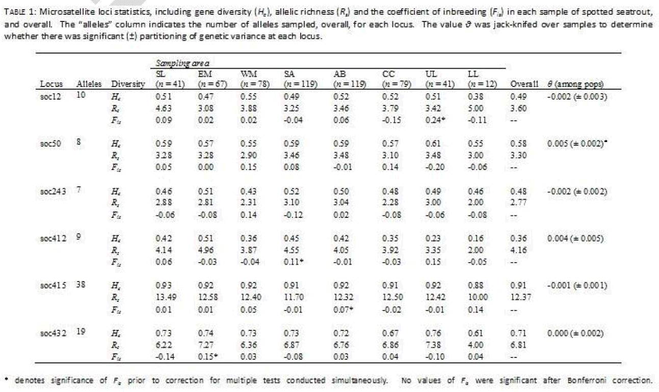
Table 1: Microsatellite loci statics, including gene diversity(H_e),allelic richness (R_e) and the coefficient of inbreeding (F_in) in each sample of spotted seatrout and overall.The “alleles”column indicates the number of alleles sampled, overall, for each locus.he value ν was jack-knifed over samples to determine whether there was significant of genetic variance at each locus.

The program FSTAT v2.9.3.2 [17] was used to measure microsatellite diversity statistics including allelic richness (R_s, [18]), gene diversity (He), the coefficient of inbreeding within samples (Fis), as well as the fixation index among all samples (θ). Additionally, FSTAT was used to test for significant genetic linkage between pairs of microsatellites using data randomization [17] with an arbitrary cutoff of α = 0.05. The statistics Fis and θ were determined initially using the methodology of Weir and Cockerham [19]. The standard error of the fixation index (θ) was determined by jackknifing over samples, and was used to determine whether there was statistical support for heterogeneity among samples at each locus. The coefficient of inbreeding (F_is) was used to determine whether there was any indication of non-random allelic associations within samples. Randomization tests were performed with 1000 iterations in order to determine whether F_is differed significantly from 0.0, which could indicate deviation from Hardy-Weinberg genotypic expectations caused either by unsampled null alleles, by differential amplification of alleles or otherwise systemic errors in allele size calling for a give locus. The nominal level for statistical significance in randomizations was adjusted for multiple tests performed simultaneously (α = 0.001).

As with the mtDNA data set, microsatellites were used in a distance-based AMOVA [9]. Initial examination of this data set revealed homogeneity among cohorts sampled in different years. Cohorts from all three years were thus pooled into single samples for spatial analyses. Variance in nuclear genotype association was partitioned into between-individual, among-sample and among-group effects using ARLEQUIN v3.0. The distance metric chosen for microsatellite AMOVA was the average number of pair wise allelic differences between individual genotypes. The same four population models used in mtDNA AMOVA were tested with the microsatellite AMOVA. Additionally, a Mantel matrix correlation analysis was used to examine isolation-by-distance of microsatellites and compared to the mtDNA Mantel test. Genetic divergence between pair wise samples was estimated (F_st) and subsequently compared to geographic distance in a matrix correspondence test as implemented in ARLEQUIN v3.0. The significance of the regression coefficient of matrix correspondence (r) was assessed by a 1000 iterations of a randomization procedure, as implemented in ARLEQUIN v3.0. Finally, a cluster analysis was performed in order to simultaneously test for number of groups (subpopulations) and group membership. For the microsatellite cluster analysis, the Cavalli-Sforza chord measure [20] was generated using PHYLIP 3.63, and the dissimilarity matrix of chord distances was subjected to Ward’s minimum-variance linkage clustering. As with the mtDNA data set, clustering was carried out using the JMP 7.0.1 software, and statistical support for nodes was obtained by bootstrap resampling in PHYLIP 3.63.

Spatial abundance of spotted seatrout in Texas

Spotted seatrout occurred ubiquitously along the Texas shoreline during the duration of TPWD sampling. Of 1,806 grids sampled, 1,785 contained spotted seatrout on at least one occasion, for an overall occurrence ratio of 0.99 (Table 2). Average CPUE among all estuaries was 0.58 (± 0.12) and ranged from 0.21 (SL) to 0.94 (LL). It is important to note that heterogeneity between spring and fall gill net spotted seatrout CPUE has been anecdotally reported, but was not explicitly examined here. The coast-wide CPUE of 0.58 represents the average among all grids, in both seasons.

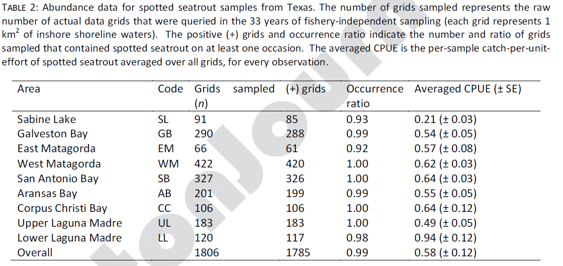
Table 2: Abundance data for spotted seatrout samples from Texas. The number of grids sampled represents the raw number of actual data grids that were queried in the 33 years of fishery-independent sampling (each grid represents 1 km² of inshore shoreline waters). The positive (+) grids and occurrence ratio indicate the number and ratio of grids sampled that contained spotted seatrout on at least one occasion. The averaged CPUE is the per-sample catch-per-uniteffort of spotted seatrout averaged over all grids, for every observation.

Qualitative observation of localized abundance indicated five areas of relatively low or ambiguous spotted seatrout abundance. The first area (area #1, Fig. 2a) was in the upper coast between SL and the unsampled Galveston bay (GB). In this area, there is not a substantial natural inshore waterway or bay area, and the Gulf Intracoastal Waterway (ICWW) represents the only inshore route of migration between SL and GB. The routine monitoring of TPWD does not set gill nets in the ICWW, so there is no estimation of abundance in this area. However, the absence of natural inshore waterways represents a physical bottleneck, and for the purpose of this project, it will be assumed such areas represent a possible dispersal or migration barrier. A second area of low/ambiguous abundance occurs between GB and EM (area #2, Fig. 2a). This is another area where inshore waterways are limited, and the ICWW represents the only substantial dispersal route for inshore species. Because GB was not sampled in this study, boundary areas #1 and #2 will be considered interchangeable for the purpose of this study, and limitations of genetic dispersal in this area will be tested by assuming that the SL sample represents a distinct subpopulation.

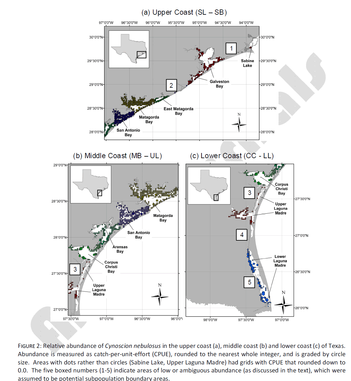
Figure 2: Relative abundance of Cynoscion nebulosus in the upper coast (a), middle coast (b) and lower coast (c) of Texas. Abundance is measured as catch-per-unit-effort (CPUE), rounded to the nearest whole integer, and is graded by circle size. Areas with dots rather than circles (Sabine Lake, Upper Laguna Madre) had grids with CPUE that rounded down to 0.0. The five boxed numbers (1-5) indicate areas of low or ambiguous abundance (as discussed in the text), which were assumed to be potential subpopulation boundary areas.

Between EM and CC (i.e. “mid-coast”), there is little evidence of low abundance in any single area (Fig. 2b). The midcoast area is characterized by large natural waterways that act as corridors between adjacent bays, in addition to the ICWW. Spotted seatrout abundance in this area is homogeneous and thus no putative subpopulation boundaries were tested in this area. In contrast, from CC south to LL there are three areas of low/ambiguous abundance. The first (area #3, Fig. 2b, 2c) is located at the northern end of UL. Despite a large natural inshore waterway between UL and CC, this area has the lowest overall abundance of any inshore area measured, and contains several adjacent grids where CPUE rounded down to 0.0. The northern UL is characterized by hyper salinity most of the year (as is the entire Laguna Madre) and extremely shallow water (~ 1-2 m, on average). Limitations of genetic dispersal in this area will be tested by assuming that Laguna Madre samples (UL + LL) together form a distinct subpopulation. A fourth low/ambiguous abundance area is between UL and LL (area #4, Fig. 2c). This is another area where there is no natural waterway, and the ICWW represents the only means of dispersal. Limitations of genetic dispersal in this area will be tested by assuming that the LL sample is its own distinct subpopulation. Finally, multiple localized areas of low abundance are present in the LL (area #5, Fig. 2c). Independent tests of divergence among multiple LL samples was not possible because sample sizes from this bay were small (n = 27 mtDNA, n = 12 microsatellite DNA) and were distributed around the entire system.

Mitochondrial DNA haplotype data

The data set used in this study was identical to the data from [6], however a brief overview of the data will be given here. Sample sizes ranged from 27 individuals (LL, WM) to 44 individuals (SL, Table 3) sequenced for a portion of the mtDNA control region. The overall mtDNA sequence set included 280 examined individuals, sequenced over 373 nucleotides, and resulted in recovery of 60 novel haplotypes. There was no evidence for heterogeneity in base frequencies among haplotypes, and the rate of transitions/transversions across a range of pair wise genetic distances indicated no evidence for mutation saturation. Among sampling sites, haplotype diversity (H_d) ranged from 0.754 (SL) to 0.940 (WM) (Table 3). Nucleotide diversity ranged from 0.005 (SL) to 0.007 (EM, WM, SB, CC, LL). There was no indication of heterogeneity among annual samples taken at the same location, thus cohorts were combined for spatial analyses.

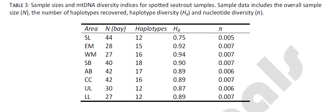
Table 3: Sample sizes and mtDNA diversity indices for spotted seatrout samples. Sample data includes the overall sample size (N), the number of haplotypes recovered, haplotype diversity (H_d) and nucleotide diversity (π).

The AMOVA procedure was used to test group (subpopulation) structure of spotted seatrout samples, using four different models derived from qualitative examination of spotted seatrout abundance (Table 4a). The model which assumed that each sampled bay harbored its own distinctive spotted seatrout subpopulation resulted in a small and statistically non-significant value of among-group structure (Φ_st = 0.011, p = 0.095). All other models, in which the midcoast bays (EM through CC) were grouped together, resulted in significant among-group structure. Of these, the model (SL) + (EM, WM, SB, AB, CC) + (UL, LL) captured the highest among-group divergence (Φ_st = 0.030) and achieved the highest statistical support (p = 0.003). This model assumed that the SL sample and both Laguna Madre samples (UL+LL, combined) came from independent subpopulations (all mid-coast samples came from a single population). Additionally, there was significant evidence of IBD, coast wide. The Mantel test indicated a strong and significant correlation between geographic distance (km) and genetic divergence (Φ_st) of mtDNA haplotypes among samples (r = 0.717, p = 0.010).

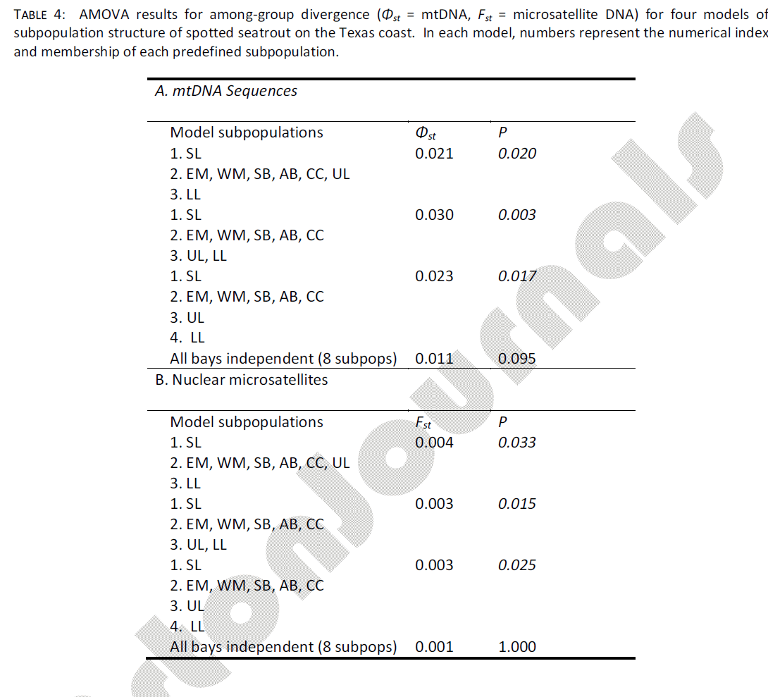
Table 4: AMOVA results for among-group divergence (Φst = mtDNA, Fst = microsatellite DNA) for four models of subpopulation structure of spotted seatrout on the Texas coast. In each model, numbers represent the numerical index and membership of each predefined subpopulation.

Multivariate cluster analysis also indicated three groups of samples. Qualitative assessment of the elbow criteria indicated that the level of clustering containing three main clusters accounted for 64% of the genetic distance assayed (Fig. 3). The first sample group to separate from all others included only the SL sample. In the second level of clustering, the UL and LL samples separated from all others, leaving the final mid-coast grouping of EM, WM, SB, AB and CC. These groupings were consistent with those that achieved the highest and most significant genetic divergence in AMOVA analyses. Bootstrap support for the mid-coast and Laguna Madre nodes were 100%.

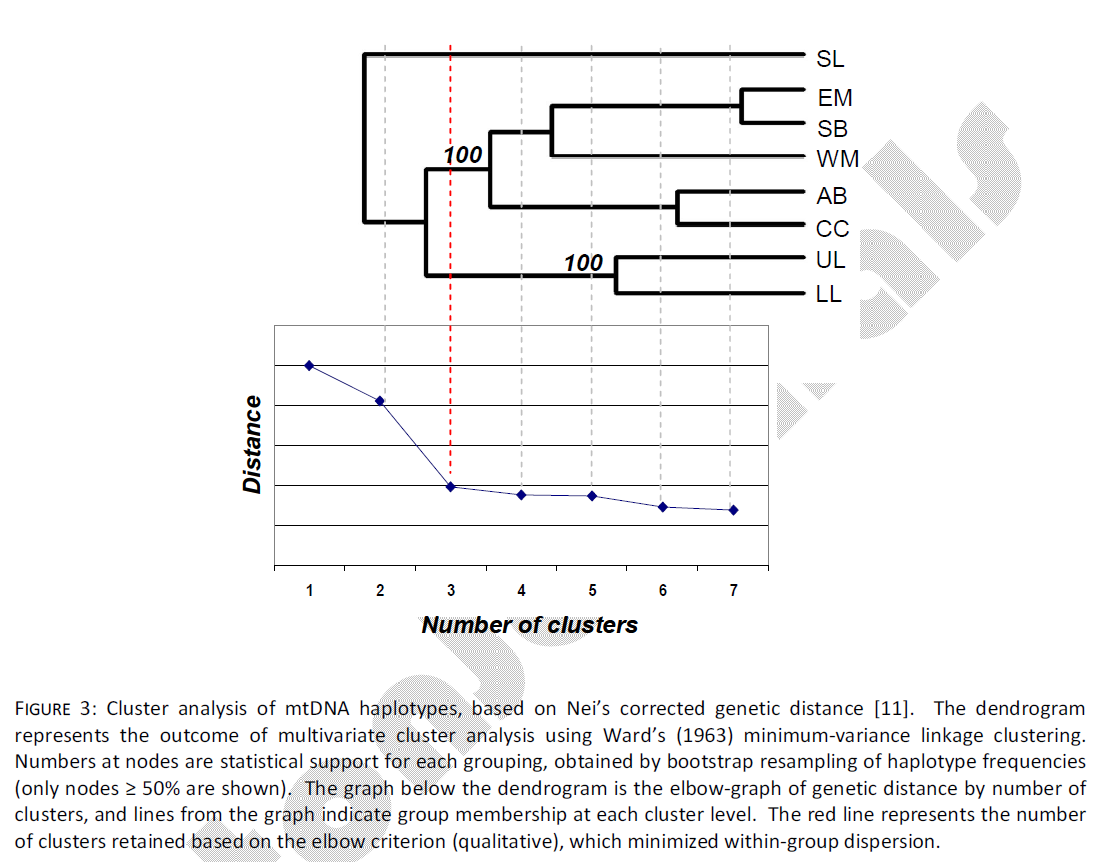
Figure 3: Cluster analysis of mtDNA haplotypes, based on Nei’s corrected genetic distance [11]. The dendrogram represents the outcome of multivariate cluster analysis using Ward’s (1963) minimum-variance linkage clustering. Numbers at nodes are statistical support for each grouping, obtained by bootstrap resampling of haplotype frequencies (only nodes ≥ 50% are shown). The graph below the dendrogram is the elbow-graph of genetic distance by number of clusters, and lines from the graph indicate group membership at each cluster level. The red line represents the number of clusters retained based on the elbow criterion (qualitative), which minimized within-group dispersion.

Microsatellite DNA data

For the microsatellite dataset the number of alleles per locus ranged from seven (soc243) to 38 alleles (soc415, Table 1). Overall allelic richness (relative variability corrected for sample size) ranged from R_s = 2.77 (soc243) to R_s = 12.37 (soc415), while overall gene diversity ranged from H_e = 0.36 (soc412) to H_e = 0.91 (soc415). In four cases, there was evidence for single locus deviation from Hardy Weinberg expectations, in single populations, as demonstrated by significantly high (> 0) values of F_is. However, in each case these values were not significant following correction for multiple tests run simultaneously. Nor was there significant evidence for linkage between any two pairs of loci. Finally, there was little evidence for heterogeneity in allele distributions among samples at individual loci. Only a single locus (soc50) had a fixation index among populations which was significantly different from 0.0 (θ = 0.005 ± 0.002).

As in mtDNA analyses, samples were grouped using the four different models derived from qualitative examination of spotted seatrout abundance (Table 4b). The model which assumed that each sampled bay harbored its own distinctive spotted seatrout subpopulation resulted in a small and statistically non-significant value of among-group structure (F_st = 0.001, p = 1.000), which was further supported by a statistically significant fixation index at only a single locus (soc50, Table 1). In addition, similar to mtDNA data, all other models tested resulted in significant among-group structure. Of these, the model (SL) + (EM, WM, SB, AB, CC) + (UL, LL) captured the 2_nd highest among-group divergence and achieved the highest statistical support (F_st = 0.003, p = 0.015). The model which considered UL to be part of the mid-coast subpopulation (SL) + (EM, WM, SB, AB, CC, UL) + (LL) achieved the highest level of among-group divergence, but had relatively weak statistical support (F_st = 0.004, p = 0.033). One possible explanation for the weak statistical support of this model is that the LL sample was the smallest of all samples taken (n = 12); this result should therefore be treated with caution.

Multivariate cluster analysis indicated the presence of three groups using microsatellite data. These three groups accounted for 75% of the genetic distance measured (Fig. 4). However, in contrast to the mtDNA data, microsatellite data indicated that the UL sample separated from all others at the first level of clustering. At the second level of clustering, the SL sample separated from all others, leaving a final grouping of EM, WM, SB, AB, CC and LL, with 95% bootstrap support. Heterogeneity in genetic dispersion within groups leveled off after the second cluster level.

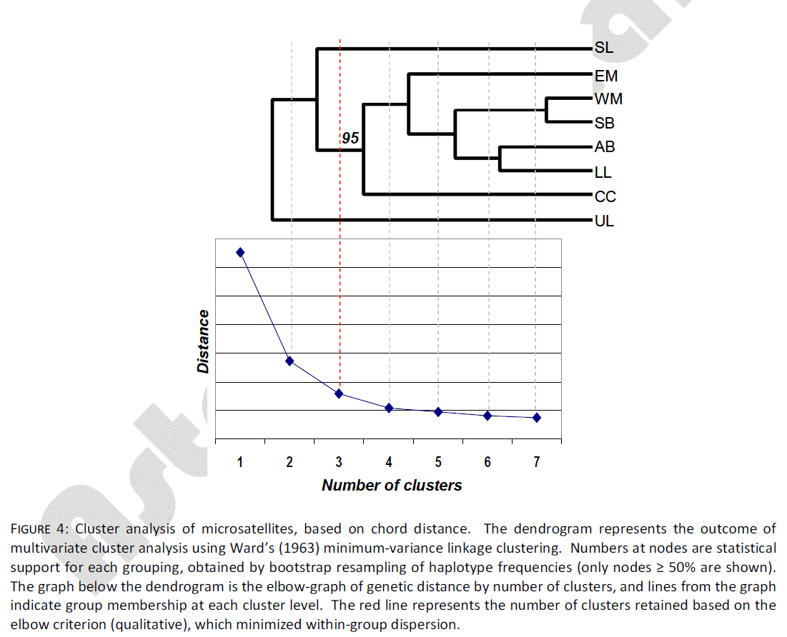
Figure 4: Cluster analysis of microsatellites, based on chord distance. The dendrogram represents the outcome of multivariate cluster analysis using Ward’s (1963) minimum-variance linkage clustering. Numbers at nodes are statistical support for each grouping, obtained by bootstrap resampling of haplotype frequencies (only nodes ≥ 50% are shown). The graph below the dendrogram is the elbow-graph of genetic distance by number of clusters, and lines from the graph indicate group membership at each cluster level. The red line represents the number of clusters retained based on the elbow criterion (qualitative), which minimized within-group dispersion.

Similar to the mtDNA data, there was significant evidence of IBD from the microsatellite data. The Mantel test of microsatellite genotype data indicated a strong and significant correlation between geographic distance (km) and genetic divergence (F_st) among samples (r = 0.617, p = 0.034).

The main intent of this study was to address two questions: 1) are there areas of chronically low abundance of spotted seatrout on the Texas coast, and 2) do spotted seatrout samples among these areas demonstrate significant discontinuity in the distribution of genetic variability. The data from this study indicate that there are areas along the Texas shoreline that indeed have chronically low abundance of spotted seatrout (such as the northern UL). Additionally, inshore waterways between adjacent bays on the northern (SL, GB) and southern (UL, LL) Texas coast consist only of the ICWW, which is of ambiguous suitability for sustaining high levels of gene flow between distant estuaries. While the middle-coast area of Texas (EM – CC) demonstrates continuously high abundance from north to south, sampling areas in the northern (SL) and southern (UL, LL) extremes resulted in higher spatial variability of spotted seatrout abundance. The low abundance of spotted seatrout in the northern UL, as well as the lack of natural inshore waterways north and south of GB, and between UL and LL, could represent areas where bay-to-bay dispersal is relatively low. For this reason, these areas may be intuitively regarded as possible subpopulation boundary areas. However, one possible caveat to this finding is that the data that was used to characterize putative subpopulation boundaries was limited in scope to areas that could support deployment of a large gill net. Thus, the differences in geospatial abundance described by this data might also be influenced by limitations of the TPWD routine monitoring sampling strategy.

Regarding the second question of discontinuity in the distribution of genetic variability among regions, results from both mtDNA control region sequences and microsatellites suggest the potential for multiple subpopulations of spotted seatrout in Texas’ coastal waters. Spatial abundance analysis results in a more systematic assessment of testable subpopulation boundaries, which in turn results in more statistically robust AMOVA results than those attained in the previous study by the authors using the same data [6]. Additionally, the cluster analyses, in contrast to AMOVA, allowed group membership to be quantitatively assigned. In particular, the benefit of multivariate clustering is that the number of groups (or subpopulations, k) and the sample membership in each group can be simultaneously assessed, without the need for group assignment a priori. Both mtDNA and microsatellite cluster analyses indicate subpopulation structure that is generally consistent with landscape abundance results. This contradicts the previous assertion that significant genetic distances at the extreme ends of a single IBD population alone were driving significant AMOVA results for Texas spotted seatrout [6].

Operating under the assumption that discreet subpopulations of spotted seatrout may exist within the territorial waters of Texas, microsatellite and mtDNA data are consistent on three points. First, the SL sample, which is the northernmost sample location, is divergent from southern samples. Both markers indicate significance of among-subpopulation AMOVA when SL is treated independently, and SL is indicated in cluster analyses as being independent from other samples. Second, there is some indication that UL and LL, the southernmost groups, also represent discreet subpopulation(s). However, the composition of subpopulation structure in the Laguna Madre samples differs between marker types. Evidence from mtDNA suggests that the UL and LL make up a single discreet subpopulation, independent from all others. This assertion is supported both by AMOVA and cluster analysis. In contrast, while microsatellite AMOVA supports the continuity of the Laguna Madre samples (UL+LL), cluster analysis indicates that the UL sample is independent of the LL sample, which clusters with mid-coast bays. One problem with this result is the microsatellite sample size for this sample; the LL microsatellite sample was by far the smallest sample taken in this study (n = 12). The Cavalli-Sforza chord measure distance method used for clustering microsatellites is allele frequency-based [20]. Therefore, it is likely that the small sample size of LL resulted in poor estimation of allele frequencies in the LL sample, which in turn resulted in ambiguous results in the cluster analysis. The mtDNA sample taken for this site was much larger (n = 27) and indicated continuity of the Laguna Madre. Finally, agreement between the two data sets indicates continuity of mid-coast regions, from EM to CC. In the case of clustering, the mid-coast samples all clustered together in the final level of clustering, whereas no genetic distances among mid-coast samples were significant in pair wise tests.

The magnitude of genetic divergence measured among putative subpopulations of spotted seatrout in this study is much higher as measured by mtDNA than that measured by microsatellite DNA. The model-based divergence between subpopulations as measured with mtDNA haplotypes (0.021< Φ <0.030) is an order of magnitude higher than the divergence measured with microsatellites (0.003< F_st <0.004). The difference between nuclear and mtDNA estimates of genetic divergence has now been consistent across a number of studies. Prior microsatellite examinations of spotted seatrout were unable to obtain consistent statistical support for divergence among Gulf subpopulations [7,8]. The magnitude of divergence among Texas populations in these studies was measured between 0.0< θ < 0.015 (range across loci, [7]), and was not significant at any locus. In contrast, a prior estimate of divergence among western Gulf localities using mtDNA was Φ_st = 0.025 (p < 0.001) [3]. The difference between nuclear and mtDNA estimates of divergence could be influenced by different genetic effective size (N_e) or migration rate (m) among males and females. In the case of N_e, the effective size of mtDNA is naturally one quarter of the effective size of nuclear DNA, because of the maternal origin of all mtDNA molecules (assuming 50/50 ratio of males/females) in combination with the haploid nature of mitochondrial genomes. If the ratio of males/females is skewed towards males, or if there is higher variance of reproductive success of females in comparison to males, this will result in an even smaller effective size of mtDNA (and presumably, elevated divergence). For instance, variance in reproductive success was suggested to play a role in dramatic differences between the genetic effective sizes of two closely related sciaenids in the western Gulf (C. nothus, C. arenarius [21]), and has been used to explain the disparity between effective population size and census size in the closely related Sciaenops ocellatus [22]. Finally, if gene flow (m) is primarily male-mediated in spotted seatrout, this will also result in a lower level of measured genetic divergence at nuclear loci. Limited female dispersal from natal areas has likely affected divergence at mtDNA loci [3]. Limited dispersal is also supported by tagging studies in Texas [23], although it is unclear whether there are differences in magnitude between male and female movements. A final possible explanation for the disparity between mtDNA and microsatellite divergence is that divergence measured by microsatellites is often influenced negatively by microsatellite polymorphism [24]. For instance, an inverse relationship between F_st and both allele richness and heterozygosity was previously demonstrated in the marine fish walleye pollock Theragra chalcogramma [25]. This effect could lead to uncertainty in interpreting significant population differentiation at microsatellite loci, as biological processes leading to divergence are difficult to disentangle from the evolutionary mechanics of microsatellite mutation [26].

The results of this study suggest different management implications than those of Anderson and Karel [6], which reached the conclusion that spotted seatrout in Texas were members of a single continuous population, with limited (intrinsic or extrinsic) barriers to dispersal. In an attempt to place spotted seatrout in Texas into one of three theoretical models described by Laikre et al. [27], Anderson and Karel [6] suggested that “continuous change” was more suitably supported by the data than discrete subpopulations. Indeed, strong clinal gradients in allozyme allele frequencies [5,28] and mtDNA haplotypes [3,6] have been found in this species. However, the population criterion of Laikre et al. [27] must be viewed as existing on a continuum between no differentiation on one end, and strong allopatric isolation of distinctive groups on the other. Spotted seatrout exist somewhere in the middle of that continuum, and on local scales, the substructure of these populations is likely affected both by isolation-by-distance (IBD), as well as by some restricted local migration among adjacent sites (Fig. 5). This is most consistent with the model hypothesized by Gold et al. [7], who suggested that spotted seatrout exist in a series of overlapping subpopulations with sufficient migration as to prevent accumulation of significant genetic divergence. The evidence from the current data further predict that there may be areas on the coast of Texas in which small-scale migration is fairly limited; it is not clear what restricts migration, but as previously mentioned there is some evidence for natal fidelity for inshore areas (primarily of females), which may be reinforced by encounters with areas of low habitat suitability (such as the northern UL).

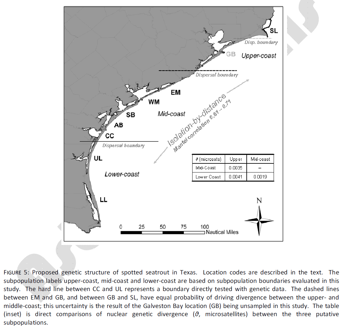
Figure 5: Proposed genetic structure of spotted seatrout in Texas. Location codes are described in the text. The subpopulation labels upper-coast, mid-coast and lower-coast are based on subpopulation boundaries evaluated in this study. The hard line between CC and UL represents a boundary directly tested with genetic data. The dashed lines between EM and GB, and between GB and SL, have equal probability of driving divergence between the upper- and middle-coast; this uncertainty is the result of the Galveston Bay location (GB) being unsampled in this study. The table (inset) is direct comparisons of nuclear genetic divergence (θ, microsatellites) between the three putative subpopulations.

This results in a more complicated model of population structure than one that can be adequately characterized by one of Laikre’s aforementioned categories. Given this complexity, some general management implications for spotted seatrout in the western Gulf that are supported by this study, as well as previous studies, will be outlined here.

First, multiple studies agree that populations of spotted seatrout in the Laguna Madre represent a demographically independent stock. King and Pate’s [5] phenogram of genetic similarity based upon allozyme data suggested that samples taken in the UL and LL region were more similar to a sample from Mexico than any samples further north. Subsequently, Gold et al. [3] indicated notable “steps” in mtDNA haplotype diversity in this area as well, and both data sets in this study support this finding. Texas Parks and Wildlife Department life history data indicate a decline in overall abundance and spawning stock biomass in LL, compared to gains in estuaries further north (unpublished data), suggesting some degree of demographic independence in the Laguna Madre. Currently, UL and LL are two of the four bays that are stocked through marine enhancement practices by TPWD. The current strategy is for stocked fingerlings to be released back into the same estuary from where the corresponding brood stock were originally extracted, although occasionally logistical considerations result in stocking into adjacent estuaries. Both of these scenarios are supported by the current data, which indicate continuity of the Laguna Madre. However, caution must be exercised, particularly as it pertains to the genetic effective size of released individuals in the LL. Gold et al. [3] reported haplotype diversity in LL that was lower than anywhere else in Texas was. This finding has not been repeated in this study or allozyme/microsatellite studies, but this result could be an indication that haplotype diversity is highly variable among years [6].

Second, multiple studies have now indicated genetic divergence between upper-coast estuaries (GB and SL), and estuaries further south. The microsatellite study of Ward et al. [8] indicated allele heterogeneity between the two northernmost bays and those occurring further south, although this heterogeneity differed in magnitude and significance through the three years of the study. Anderson and Karel [6] indicated dramatic haplotype frequency differences between SL and all other samples, and this is reflected in the current microsatellite data. Unfortunately, GB was not sampled in the current study. These two northernmost estuaries (GB and SL) are the remaining two estuaries into which TPWD practices marine stock enhancement. Similar to lower coast stocking, stocking practices in the upper coast dictate that fingerlings are released into the estuary from which brood stock are extracted, with consideration for logistical issues mentioned above. The current data support stocking in the bay of origin or into adjacent bays. Although it is impossible to evaluate differences between GB and SL with the current data specifically, caution must be urged for two reasons. First, the spatial abundance data presented here indicate that the ICWW is the only avenue of dispersal between these two estuaries, and it is unclear how frequently spotted seatrout use these areas as dispersal corridors, with any frequency. Second, the low intrapopulation haplotype diversity recovered in Anderson and Karel [6] may indicate that SL is demographically independent from sites further south. This clearly represents an avenue where future study is warranted.

This work was funded by two National Marine Fisheries Service Grants, through the Federal Aid in Sportfish Restoration program. Otherwise, the authors declare that they do not have any competing interests.

JA carried out all GIS tasks, mtDNA sequencing assays, statistical manipulations of both data sets, drafted the manuscript and made corrections. WK carried out all microsatellite DNA assays and assisted with analysis of microsatellite data.

We wish to thank the personnel of the Texas Parks and Wildlife Routine monitoring program for providing the samples used in genetic analyses. Heather Hendrickson assisted with laboratory tasks. Ashley Summers provided technical assistance with GIS analysis. Mark Fisher, Dusty McDonald and Britt Bumguardner as well as three anonymous reviewers improved the initial draft of the manuscript with helpful comments. TPW routine monitoring is carried out with the support of a NMFS Federal Aid in Sportfish Restoration Grant, F-34M. This research was specifically funded by NMFS Federal Aid in Sportfish Restoration Grant F-143-R.