Journal of Physical Chemistry & Biophysics
Open Access
ISSN: 2161-0398
ISSN: 2161-0398
Research - (2023)Volume 13, Issue 6
Tower solar thermal power generation technology is a new low-carbon and environmentally friendly clean energy technology. In this paper, based on Monte Carlo algorithm model and Particle Swarm Optimization (PSO) algorithm, the optimization model of heliostat mirror field is constructed, which is of great practical significance for effectively improving the collection and conversion efficiency of solar energy and promoting the sustainable development of clean energy.
First of all, this paper first visualizes the coordinate data of each heliostat attached in the spatial coordinate system, and carries out preliminary screening and cleaning of the data. Then combined with the known conditions in the topic and the formula in the appendix to determine the shadow occlusion efficiency (ηsb), cosine efficiency (ηcos), atmospheric transmittance (ηat), collector truncation efficiency (ηtrunc) and mirror reflectance (ηref) and other 5 parameter values, these parameter values into the helioscope optical efficiency calculation formula, to solve the average optical efficiency on the 21st of each month, Then the average optical efficiency of 12 months is calculated, and the average annual optical efficiency of heliostat field is 0.4512. Similarly, the average annual output thermal power of the heliostat field is calculated as 27.5713 MW by using the calculation formula of the output thermal power of the heliostat field, and then divide the annual average thermal power by the sum of the mirror areas of all heliostats in the whole field (there are 1745 heliostats, and the area of each mirror is 36 m2). Finally, the average annual output thermal power per unit mirror area is 0.4401 kw/m2.
Second, this paper uses Monte Carlo direct model and PSO algorithm to build a mathematical model of optimization design of heliostat mirror field. The mirror height is not greater than the mirror width, the mirror side length is between 2 m-8 m, the installation height is between 2 m-6 m, the mirror will not be in contact with the ground when rotating around the horizontal axis, the distance between the base centres of the adjacent two mirrors must be at least 5 m more than the width of the mirror, the helioscope is not installed in the circular area of 100 m around the endothermic tower, and the radius of the helioscope field of the whole circle is 350 m, the size parameters of each helioscope and the installation height is the same, the rated annual average output thermal power of the heliostat field is not less than 60 MW as the constraint condition, the position coordinate of the absorption tower, the size of the heliostat, the installation height, the number of heliostat and the position of the heliostat are taken as the design parameters, and the maximization of the annual average output thermal power per unit mirror area is taken as the objective function. After entering the model, the optimal design parameters are solved as follows: The position coordinate of the absorption tower is (0, -200), the size of the heliostat is 3.5 m × 3.5 m, the installation height is 2 m, the total number of the heliostat is 8440, and the total area is 103390 m2.
Finally, on the basis of step two, the helioscope installation area is divided into four ring areas. The helioscope in the same area has the same size and installation height, while the helioscope in different rings has different size and installation height, so as to effectively optimize the parameter values of truncation efficiency and shadow occlusion efficiency. The optimal design parameters in each ring can be obtained by using the established optimization model.
Monte Carlo algorithm; PSO algorithm; Heliostat field; Optimal design
Research background
Chinese government and enterprises attach great importance to tower solar thermal power generation technology. At present, China has made certain breakthroughs and achievements in tower power station technology, which is expected to play an important role in the future energy field. Tower solar thermal power station is a new type of clean energy technology using solar energy to generate electricity. It generates electricity by collecting solar energy and converting it into heat, which is then converted into electricity. Heliostat is a key device used in tower power stations to collect and track solar rays.
In the tower solar thermal power station, by combining a large number of heliostats according to a certain spatial position to form the heliostats field, the sunlight can be focused on a point, so that the sunlight can be concentrated on the heat absorber in the centre of the heliostats field. The heat absorber is usually composed of a thermal medium (such as water or molten salt), when the sun shines on the heat absorber, the thermal medium will absorb the solar energy and convert it into heat energy, and then convert from heat energy to electric energy through heat exchange.
Research restatement
Now it is planned to build a circular heliostat field in a circular area with a radius of 350 m and an altitude of 3000 m. The centre is located at 39.4° north latitude and 98.5° east longitude. Taking the centre of the circular region as the origin, the space rectangular coordinate system of the mirror field is established with the X-axis forward in the due east direction, Y-axis forward in the due north direction, and Z-axis forward in the upward direction perpendicular to the ground.
Research objective 1: The absorption tower is located in the centre of the mirror field, the side length of the heliostat is 6 m × 6 m, and the installation height is 4 m. Using this we can calculate the annual average optical efficiency of the mirror field, the annual average thermal output power and the annual average thermal output power per unit mirror area according to the position of the heliostat centre are given below, and the results are shown in the tabular form.
Research objective 2: The rated annual average output thermal power (rated power) of the heliostat field is 60 MW. Assuming that the side length size and installation height of all heliostats are the same, we can design a scheme combining the position coordinates of the absorption tower, the side length size of the heliostat, the installation height, the number of heliostats, the position coordinates of the heliostat and other parameters, so that the entire mirror field can achieve the rated power. The average annual output thermal power per unit mirror area can be maximized, and the specific results of the above parameters are shown in the tabular form.
Research objective 3: On the basis of step two, if the side length and installation height of each heliostat can be different, we can redesign each parameter so that the average annual output thermal power per unit mirror area can be maximized under the premise that the entire mirror field reaches the rated power, and the specific results of the above parameters are shown in the tabular form.
Research analysis
Analysis of research objective 1: This Research requires solving the three data of the average annual optical efficiency, average annual thermal output power and average annual thermal output power per unit mirror area of the heliostat field. According to the reference formula given in the appendix, it is necessary to the reference formula given in the appendix, it is necessary to determine the value of the shadow blocking efficiency (ηsb), cosine efficiency (ηcos), atmospheric transmittance (ηat), collector truncation efficiency (ηtrunc) and mirror reflectivity (ηref) of these five parameters as well as the number and total area of the mirror, and then bring it into the formula for solving.
Analysis of research objective 2: This Research belongs to an optimization research. The rated annual average output thermal power of the heliostat field is not less than 60 MW as the constraint condition, the position coordinates of the absorber tower, the size of the heliostat, the installation height, the number of heliostat and the position of the heliostat are taken as the design parameters, and the maximum annual average output thermal power per unit mirror area is taken as the objective function. Monte Carlo and PSO algorithm are used to construct a mathematical model for the optimal design of heliostat field, and the optimal design parameters can be solved by bringing the constraints and objective functions into the model. Analysis of research objective 3: On the basis of step two, this Research does not specify that the size and installation height of all heliostats are the same, and other constraints, objective functions and design parameters remain unchanged. In this Research, the area for installing heliostats is divided into four ring areas. The size and installation height of heliostats in the same area are the same, while the size and installation height of heliostats in different rings are different. Bringing it into the optimization model established in the second Research can solve the optimal parameter design in each ring.
Model hypothesis and symbol description
Assumptions of the model and reasons for assumptions: In the mathematical modelling of optimization design of heliostat field, in order to simplify the research and calculation process and facilitate the establishment and solution of the model, the following assumptions are made for the model: When calculating the optical efficiency, it is assumed that the reflectivity of the heliostat is constant and is not affected by the incidence Angle of the sun.
Note: This hypothesis is to simplify the complexity of the model. In the actual process, the position of the sun will change with the change of time, which will cause the incidence angle of the sun's light on the mirror to change, which may lead to the change of the reflectivity of the mirror. When calculating the optical efficiency, the influence of external factors such as mirror pollution and mirror shape change caused by high temperature on the optical performance of the heliostat is not considered.
Note: According to the information given in the title, the heliostat has the need for regular maintenance and cleaning, that is, in the actual process, the heliostat may have the research of mirror pollution and mirror shape change, which will affect the optical performance of the heliostat.
A simplified method is adopted in the calculation. The calculation time of all "annual average" indicators is taken as a specific time on the 21st day of each month in local time: 9:00, 10:30, 12:00, 13:30, 15:00, and the solar light intensity during this time period is relatively stable.
Note: This assumption is to facilitate the calculation of the model and the comparison of results, and stipulates that the calculation time of all "annual average" indicators is a specific time on the 21st day of each month. This assumption can make the final calculation results comparable and consistent.
Symbol description: In the mathematical modelling for the optimization design of heliostat field, in order to facilitate the code writing, the general symbols of the full text are described as follows in Table 1.
| Symbol | Meaning description | Unit |
|---|---|---|
| αs | Solar altitude angle | |
| γs | Solar azimuth | |
| φ | Local latitude | Degree (°) |
| ω | Solar hour Angle | Degree (°) |
| δ | Solar declination Angle | Degree (°) |
| ST | Local time | Hour and minute |
| a | The horizontal coordinate of the tower | |
| b | The vertical coordinates of the tower | |
| xi | The horizontal coordinate of the I-th mirror | |
| yi | The vertical coordinates of the I-th mirror | |
| D | The number of days until the vernal equinox | |
| DNI | Normal direct radiation irradiance | KW/m2 |
| G0 | Solar constant | KW/m2 |
| h | Mirror height | m |
| d | Mirror width | m |
| l | Mirror mounting height | m |
| H | Altitude | KM |
| Ha | Height of absorber | m |
| Efield | Thermal output power of heliostat field | MW |
| E_ave | Average annual thermal output per mirror area | KW/m2 |
| Ai | Daylighting area of the I-heliostat | m2 |
| ηi | Optical efficiency of the I-mirror | |
| ηsb | Shading efficiency | |
| ηcos | Cosine efficiency | |
| ηat | Atmospheric transmittance | |
| ηtrunc | Collector cut-off efficiency | |
| ηref | Specular reflectance | |
| dHR | Distance from the centre of the mirror to the centre of the collector | m |
Table 1: Description of symbols.
The establishment and solution of the model
Establishment and solution of research 1 model: Data cleaning- in this paper, the coordinates of the heliostat given in the attachment are visually displayed in the space coordinate system in the form of particle points by using MATLAB software, as shown in the following Figure 1.

Figure 1: Visualization of the spatial position distribution of each heliostat in the mirror field.
As seen from Figure 1, the heliostats in the mirror field basically show a ring shape and are evenly distributed in the mirror field. Then, taking no heliostat installed within 100 m around the absorption tower as the constraint condition, combined with the space coordinate system established in the background of the topic, taking the tower as the central origin, the coordinates of each heliostat in the attachment were calculated by using the Euclidean distance formula to determine whether the distance between them and the tower met the constraint conditions to clean the data. Through calculation, it was concluded that the data in the attachment met the constraint conditions.
Model establishment known conditions
Geographical location of the mirror field: The whole mirror field is a circular heliostat field with a radius of 350 m. Its centre is located at 39.4° north latitude and 98.5° east longitude, with an altitude of 3000 m.
The establishment of the rectangular coordinate system of the mirror field space: The centre of the mirror field is the origin, the due east direction is the x axis forward, the due north direction is the y axis forward, and the upward direction perpendicular to the ground is the z axis forward. The physical diagram is as follows in Figures 2 and 3.

Figure 2: Physical diagram of heliostat field. Note:  Distribution
of heliostats in the field,
Distribution
of heliostats in the field,  Absorption tower.

Figure 3: Physical model of sunlight reflected by heliostat.
The internal planning of the mirror field: The absorption tower is located in the centre of the circular mirror field, the absorption tower is 80 meters high, the collector is 8 m high and 7 m diameter of the cylinder, the side length of the heliograph is 6 m × 6 m, and the installation height is 4 m.
Constraints
• The height of the mirror is not greater than the width of the mirror.
Verification: The mirror height in this research is equal to the mirror width, which meets the constraint conditions
• The mirror side length is between 2 m-8 m.
Verification: The side length of the heliostats in this research is 6 m × 6 m, between 2 m-8 m, which meets the constraint conditions.
• The installation height is between 2 m-6 m.
Verification: The installation height of the heliostats in this research is 4 m, between 2 m-6 m, which meets the constraint conditions.
• There will be no contact between the mirror and the ground when rotating around the horizontal axis.
Verification: The mirror height of the heliostat mirror in this research is 6 m, and the installation height is 4 m. When the mirror is rotated around the horizontal axis to be completely perpendicular to the ground, there is still 1 m distance between it and the ground, which meets the constraint conditions.
• The distance between the centres of the base of the two adjacent mirrors must be at least 5 m more than the width of the mirror.
Verification: According to the data coordinates given in the attachment, the distance between the base centres of the adjacent two mirrors can be calculated by using Euclidean formula to meet the constraint conditions.
Solution objective:
• Annual mean optical efficiency of heliostat field.
• Annual average output thermal power of heliostat field.
• Annual average output thermal power per unit mirror area.
Solution of annual average optical efficiency: The optical efficiency of a heliostat is the proportion of energy that a given heliostat uses to focus sunlight on the focal point. The optical efficiency of a heliostat can be calculated by the following formula:
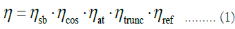
In the above formula, η represents the optical efficiency of the helioscope, ηsb is the shadow occlusion efficiency, ηcos is the cosine efficiency, ηat is the atmospheric transmittance, ηtrunc is the collector truncation efficiency, ηref is the mirror reflectance. Calculate the values of 5 parameters into the formula to solve the optical efficiency of the heliostat, the specific solution steps are as follows: The shadow occlusion efficiency ηsb is the degree to which the specified helioscope surface is obscured by shadows, and its formula is as follows:
ηsb=1-Shadow occlusion loss ……… (2)
This formula represents the proportion of energy not obscured by shadows. It can be inferred from the formula that the smaller the shadow occlusion loss, the higher the shadow occlusion efficiency, and the higher the optical efficiency of the heliostat.
The shadow occlusion loss in this paper includes three parts [1], as shown in Figure 4. The obstruction of the front arranged heliostat to the rear arranged heliostat receiving sunlight, the obstruction of the front arranged heliostat to the reflection of sunlight by the rear arranged heliostat as shown in Figure 5, and the obstruction of the tower's projection to the heliostat as shown in Figure 6.

Figure 4: Composition of shadow occlusion loss.

Figure 5: Blocking between mirrors.

Figure 6: Obstruction of tower body projection.
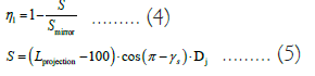
Part 1-shadow occlusion loss caused by tower body projection
Calculation of the overall height of the tower body: The title specifies that the height above the ground of the collector centre is called the height of the absorption tower. In research 1, the height of the tower is 80 m, and the height of the collector is 8 m. Therefore, the overall height of the tower is the height of the tower plus the upper half of the collector. Therefore, the overall height is 84 m. Assuming that the projection length of the entire tower is L, the calculation formula is as follows:
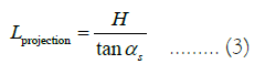
The title stipulates that there is no heliostat within a circular area of 100 m around the absorption tower, so the shadow occlusion loss caused by the projection of the tower body is only calculated when the length of the L projection exceeds 100 m. Due to the fact that the collector is a cylindrical shape, the shadow area formed by the projection of the tower can be approximated as a parallelogram. The truly effective shadow area S is the total shadow area minus the area of the shadow area with a projection length of less than 100 m. It is advisable to assume that the floor area of all heliostats in the entire mirror field is Smirror, and the shadow blocking efficiency caused by the projection of the tower is η1, then:
In Formula (5), it is the solar azimuth angle, Dj is the diameter of the collector, and Dj=7.
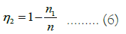
Part 2-shadow occlusion loss caused by the front and rear mirrors
Firstly, divide the mirror in the back row into n points and calculate whether each point can successfully receive and reflect sunlight, in order to calculate the shadow occlusion loss η2 for that part. Set the number of occluded points to n1.
The solving steps are as follows:
Step 1: Establishing a mirror coordinate system (Figure 7).

Figure 7: Mirror coordinate system.
Step 2: Coordinate transformation
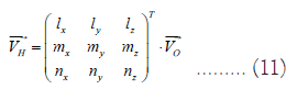
Firstly, convert the mirror coordinates of each point in the rear mirror into ground coordinates. Assuming that the unit matrix of the conversion relationship between the mirror coordinate system and the ground coordinate system is as follows:
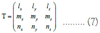
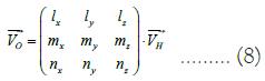
Assuming that the vector of a beam of light in the mirror
coordinate system is represented as  , and the vector in the
ground coordinate system is represented as
, and the vector in the
ground coordinate system is represented as  , then there is the
following relationship:
, then there is the
following relationship:
Assuming that there is a point on the helioscope with coordinates H1 (x1, y1, 0), first convert it to ground coordinates H2 (x2, y2, z2).
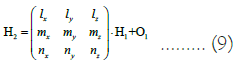
O1 is the coordinate value of the origin of the rearranging heliostat mirror coordinate system in the ground coordinate system, expressed as (x0, y0, z0).
Convert H2(x2, y2, z2) to the coordinates H3(x3, y3, z3) in the front mirror coordinate system.
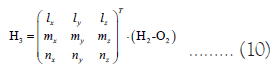
O2 is the coordinate value of the origin of the pre-arranged
heliostat mirror coordinate system in the ground coordinate
system, represented by (x4, y4, z4). The vector of light rays in
the ground coordinate system is converted to the pre-arranged
heliostat mirror coordinate system, represented by 
Step 3: Finally, based on point H3 and the principle of two points and one line, calculate the intersection point between the light and the pre-arranged helioscope, and determine whether the intersection point is within the pre-arranged helioscope.
Finally, add up the values of the three parts of shadow occlusion loss and take the average value as the final result of shadow occlusion efficiency ηsb.
The cosine efficiency ηcos is the effect of the angle between the specified heliostat mirror surface and sunlight on optical efficiency, and its calculation formula is as follows:
ηcos=1-Cosine loss ……… (12)
This formula represents the proportion of energy not lost due to the included angle; according to the formula, the smaller the included angle, the smaller the cosine loss, and the higher the optical efficiency of the heliostat. Cosine loss refers to the decrease in received energy caused by the direction of sunlight incidence not parallel to the normal direction of the mirror aperture.
Angle included in Figure 8. And the cosine value of θ is the cosine efficiency of the point (Figure 9).

Figure 8: Physical diagram of cosine efficiency.

Figure 9: Flowchart of solving cosine efficiency.
According to the definition of cosine loss, when a heliostat, collector, and the sun form a "three point line", the cosine efficiency of the heliostat will reach its theoretical maximum. The optimal method is to assume that the intersection point of the incoming rays of the sun and the mirror is the centre of the mirror, and the intersection point of the reflected rays and collector is the centre of the collector. The vector of the reflected rays can be calculated from the spatial coordinates of these two centre points; similarly, the vector of the extension line of incoming and outgoing rays can be calculated by the position of the sun and the coordinates of the centre of the mirror, and then the two vectors can be used to calculate twice the cosine value of α in Figure 8; And then calculate it through the inverse trigonometric function α and then calculate the angle of θ Angle.
The position of the sun [2], can be determined by the solar altitude of angle and the azimuth of angle αs, where the cosine value of the solar azimuth angle γs is calculated as follows:

In the formula, δ is the solar declination angle and φ is the local latitude. The vector of the extension line of the incident light can be expressed as:

Atmospheric transmittance ηat refers to the energy loss caused by sunlight passing through the atmosphere, and its calculation formula is as follows:

In the formula, dHR represents the distance from the centre of the mirror surface to the centre of the collector; According to the formula, the higher the atmospheric transmittance, the higher the optical efficiency of the heliostat; According to the spatial Cartesian coordinate system established in this research, the spatial coordinates of the collector centre are (0, 0, 80), and the spatial coordinates of the mirror centre are (x, y, 4). The coordinates of x and y are shown in the attachment. The threedimensional Euclidean distance formula can be used to solve dHR, and then the value of dHR can be brought into the above calculation formula to calculate the atmospheric transmittance ηat.
The truncation efficiency of the collector ηtrunc is the ratio between the total reflected energy of the designated heliostat mirror and the received energy of the collector, and its calculation formula is as follows:
ηtrunc=Energy received by the collector/(mirror total reflection energy-shadow occlusion loss energy) ……… (16)
Due to the fact that the sunlight is a conical beam of light with a certain conical angle [1], as shown in the Figures 10 and 11 below, the above formula can be transformed into the following formula:

Figure 10: Sun rays.

Figure 11: Optical cone coordinate system.
In the formula, mreflection is the total number of solar rays that are evenly divided by the angular mean method, and mreception is the total number of solar rays successfully received by the collector.
The solution steps are as follows:
Step1: Establish a light cone angle coordinate system and use vectors to represent each beam of light.
Step2: Convert the mirror coordinates of a point on the mirror surface to ground coordinates.
Step3: Find the vector representation of each beam of light in the ground coordinate system.
Step4: Find the vector of reflected light for each beam of sunlight in the ground coordinate system.
Step5: Determine whether each beam of light has successfully landed on the collector based on the surface equation of the collector and whether there is an intersection between the reflected rays.
Mirror reflectance-ref specifies the reflection ability of the sun mirror to sunlight. The value of ηref is closely related to the material used in heliostat. After consulting relevant literature, the value of ηref in this paper is a constant of 0.92.
Combined with the above steps, the values of shadow occlusion efficiency (ηsb), cosine efficiency (ηcos), atmospheric transmittance (ηat), collector truncation efficiency (ηtrunc) and known mirror reflectance (ηref) can be calculated after the formula (1), the optical efficiency η of the heliostatic mirror can be calculated.
Solution of annual average thermal output power
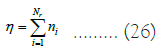
The calculation formula for the output thermal power Efield of the heliostat field is:
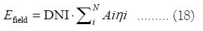
DNI is the irradiance of normal direct radiation; N is the total number of heliostats. It can be seen from the attachment that N=1745 in this paper; Ai is the lighting area of the i heliostat, Ai=36 in this research; ηi is the optical efficiency of the I-th mirror.
Normal direct radiation irradiance DNI refers to the solar radiation energy received per unit area and per unit time on a plane perpendicular to the sun's rays on Earth. The approximate calculation formula is as follows:
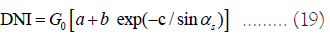
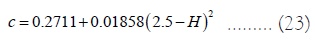
Where G0 is the solar constant, representing the intensity of solar radiation energy in the Earth's outer atmosphere. In this article, a constant value of 1.366 kW/m2 is taken, where sinαs is the sine value of the solar altitude angle αs, and the coefficients a, b, and c are calculated as follows:
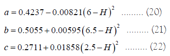
In the formula, H represents the altitude, in kilometres. Based on the background of the research, the value of H in this article can be taken as 3, which can be calculated by taking it into account:
a=0.3498,b=0.5784,c=0.2757.
The solar altitude angle αs represents the angle between the sunlight and the ground plane, and its sine value is calculated as follows:
In the formula, φ is the local latitude, in this article, φ=39.4°, ω is the solar time angle, and δ is the solar declination angle.
The formula for calculating the solar time angle ω is as follows:
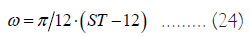
In the formula, ST is the local time. In this article, we take 9:00, 10:30, 12:00, 13:30, and 15:00 on the 21st day of each month to calculate the value of the solar time angle, as shown in the Table 2 below:
| ST | 9:00 | 10:30 | 12:00 | 13:30 | 15:00 |
| ω | -0.7854 | -0.3927 | 0 | 0.3927 | 0.7854 |
Table 2: Values of solar hour Angle.
The calculation formula for the solar declination angle δ is as follows:
sinδ = sin (2π D 365) sin (2π 360× 23.45) ……… (25)
In the formula, D is the number of days starting from the 0th day based on the vernal equinox. According to this definition, the D value of the 21st day of each month can be calculated, as shown in the Table 3 below:
| Time | 1.21 | 2.21 | 3.21 | 4.21 | 5.21 | 6.21 |
| D | 306 | 337 | 0 | 31 | 61 | 92 |
| Continue table: | ||||||
| Time | 7.21 | 8.21 | 9.21 | 10.21 | 11.21 | 12.21 |
| D | 122 | 153 | 184 | 214 | 245 | 275 |
Table 3: D values of 21 days of each month.
After incorporating the D value of the 21st day of each month into the formula for calculating the solar declination angle δ, the solar declination angle δ of the 21st day of each month can be calculated.
δ in the following table is expressed in radians:
By combining the data from Tables 3 and 4 and using the calculation formula for calculating the output thermal power of the heliostat Efield, the thermal output power of each month at five specific times on the 21st can be calculated. Then, the average of the five thermal output powers of each month can be calculated to obtain the monthly average thermal output power. Then, the average of the 12 monthly average thermal output powers can be summed up to obtain the annual average thermal output power. The specific results are shown in Tables 5 and 6.
| Time | 1.21 | 2.21 | 3.21 | 4.21 | 5.21 | 6.21 |
| δ | -0.3450 | -0.1855 | 0 | 0.2038 | 0.3525 | 0.4092 |
| Continue table: | ||||||
| Time | 7.21 | 8.21 | 9.21 | 10.21 | 11.21 | 12.21 |
| δ | 0.3506 | 0.1947 | -0.0103 | -0.2068 | -0.3578 | -0.4092 |
Table 4: The declination Angle of the sun on 21st of each month.
| Date | Average Optical efficiency | Average cosine efficiency | Average Shadow Occlusion Efficiency | Average truncation efficiency | Average output thermal power per unit area mirror (kw/m2) |
|---|---|---|---|---|---|
| January 21st | 0.4428 | 0.7617 | 0.898 | 0.7464 | 0.4341 |
| February 21st | 0.446 | 0.7761 | 0.9175 | 0.7579 | 0.4333 |
| March 21st | 0.4508 | 0.7563 | 0.8929 | 0.7589 | 0.4399 |
| April 21st | 0.4582 | 0.7349 | 0.9019 | 0.7576 | 0.4481 |
| May 21st | 0.4584 | 0.7603 | 0.8935 | 0.7563 | 0.4372 |
| June 21st | 0.4438 | 0.7605 | 0.8953 | 0.7554 | 0.4451 |
| July 21st | 0.4585 | 0.7554 | 0.9218 | 0.7547 | 0.4351 |
| August 21st | 0.4582 | 0.7511 | 0.9171 | 0.7544 | 0.4444 |
| September 21st | 0.4497 | 0.7667 | 0.9033 | 0.7433 | 0.4357 |
| October 21st | 0.4554 | 0.7756 | 0.9264 | 0.7484 | 0.4401 |
| November 21st | 0.4436 | 0.7705 | 0.893 | 0.7497 | 0.4435 |
| December 21st | 0.4486 | 0.7627 | 0.9078 | 0.7406 | 0.4469 |
| January 21st | 0.4428 | 0.7617 | 0.8980 | 0.7464 | 0.4341 |
| February 21st | 0.4460 | 0.7761 | 0.9175 | 0.7579 | 0.4333 |
| March 21st | 0.4508 | 0.7563 | 0.8929 | 0.7589 | 0.4399 |
| April 21st | 0.4582 | 0.7349 | 0.9019 | 0.7576 | 0.4481 |
| May 21st | 0.4584 | 0.7603 | 0.8935 | 0.7563 | 0.4372 |
| June 21st | 0.4438 | 0.7605 | 0.8953 | 0.7554 | 0.4451 |
| July 21st | 0.4585 | 0.7554 | 0.9218 | 0.7547 | 0.4351 |
| August 21st | 0.4582 | 0.7511 | 0.9171 | 0.7544 | 0.4444 |
| September 21st | 0.4497 | 0.7667 | 0.9033 | 0.7433 | 0.4357 |
| October 21st | 0.4554 | 0.7756 | 0.9264 | 0.7484 | 0.4401 |
| November 21st | 0.4436 | 0.7705 | 0.8930 | 0.7497 | 0.4435 |
| December 21st | 0.4486 | 0.7627 | 0.9078 | 0.7406 | 0.4469 |
Table 5: Average optical efficiency and output power on 21 days per month in Research.
| Average optical efficiency | Average cosine efficiency | Average Shadow Occlusion efficiency | Average Truncation efficiency | Annual average thermal power output (MW) | Annual average output of mirror surface per unit area Thermal power (kw/m2) |
|---|---|---|---|---|---|
| 0.4512 | 0.7564 | 0.9057 | 0.7519 | 27.5713 | 0.4401 |
Table 6: Annual average optical efficiency and output power table.
Solving the annual average output thermal power per unit mirror area
By dividing the average monthly thermal output power of the heliostat in above solution by the mirror area of the total heliostat, the average monthly thermal output power per unit mirror area can be obtained. After calculating the average monthly thermal output power per unit mirror area for 12 months, the average annual thermal output power per unit mirror area can be obtained.
In this small research, the total number of mirrors is 1475, the area of each mirror is 36 m2, multiply the two, there can solve the total heliostat mirror area.
Summary of research 1 solution results
After performing data visualization operations on the data in Table 5 and Figure 12, it was found that the average shadow occlusion efficiency was the highest during the summer solstice period. The possible reason is that during the summer solstice, the sun is located near the Tropic of Cancer, and the geographical location of the mirror field is 39.4 degrees north latitude. At this time, the projection length generated by direct sunlight on the tower is the smallest, so the average shadow occlusion efficiency is the highest.

Figure 12: Visualize data in Table 5. Note:  Average cosine
efficiency,
Average cosine
efficiency,  Average optical efficiency,
  Average shadow
occlusion efficiency,
Average shadow
occlusion efficiency,  Average truncation efficiency.
Establishment and solution of research 2 model
Model proposal: The optimization design of the heliostat field in tower solar thermal power generation systems can effectively improve the efficiency of solar energy collection and conversion. We use a direct model based on Monte Carlo algorithm and combined with PSO algorithm to solve the optimization design research of the average output thermal power per unit mirror area of a heliostat.
Monte Carlo algorithm: Monte Carlo algorithm is a numerical calculation method based on random sampling. It constructs a probability model with similar performance to the model to be solved, conducts random sampling and statistical experiments on this probability model, and obtains specific numerical features through the sampling results. In this algorithm, the value of the objective function is estimated through randomly generated sample points.
PSO algorithm: PSO algorithm is a heuristic optimization algorithm that simulates the behaviour of groups such bird or fish schools. In the PSO algorithm, each particle represents a potential solution to the research, corresponding to a fitness value determined by the fitness function. Each individual (particle) updates their position and velocity by learning their own and group experiences. The velocity of the particle determines the direction and distance of the particle's movement, and the velocity dynamically adjusts with the movement experience of themselves and other particles, thus achieving the individual's search for the optimal solution in the solvable space.
Selection of coordinate system: The arrangement method of the heliostat field in this study is to increase the annual average output thermal power per unit mirror area through staggered arrangement of heliostats [3]. Since the position of the absorption tower does not affect the layout of the heliostat, the coordinates of the absorption tower are taken as the origin of the fixed value to establish a spatial Cartesian coordinate system, as shown in the following, Figure 13.

Figure 13: Schematic diagram of establishing a spatial coordinate system.
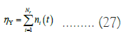
Calculation of instantaneous heliostat field efficiency
The optical efficiency of the instantaneous heliostat field is calculated by the average efficiency Nr, and the formula for solar radiation is as follows:
Sampling light over a period of one year and passing the average efficiency Nr, solar light is a symbol of time, and the optical efficiency of the annual heliostat field is:
Using models to simulate typical annual cycles to track the position of the sun. The heliostat reorients the geometric shape of the SPT based on the position of the sun in the sky.
Establishment of an optimization model for heliostats
This research aims to maximize the annual average output thermal power per unit mirror area of the heliostat field under the condition of reaching the rated power. Based on the first research, with the annual average output thermal power per unit mirror area as the target, the following model is constructed using formulas (1), (5), (9), and (16):
Constraint condition:
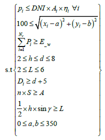
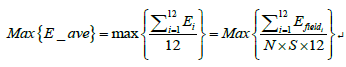
Objective function:
Solution of the optimization model for heliostats
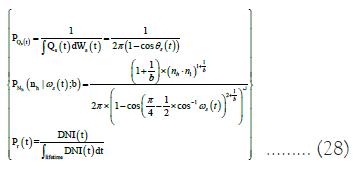
Probability density function and Monte Carlo weight with time variation: The system is initialized to the cosine loss, solar angle, and other auxiliary function results solved by the first research, and the optimal solution is found through random search and analysis. The Monte Carlo algorithm is used to simulate the optical efficiency of a heliostat, estimating the average output thermal power per unit area through random sampling, and the PSO algorithm is used to optimize the design parameters of the heliostat to maximize the average output thermal power per unit area (Figure 14).

Figure 14: Physical schematic diagram of using Monte Carlo algorithm to track solar rays.
Firstly, a DNI is calculated based on p (t) and retained for 1 hour
during its lifecycle. Then, a uniform sampling Q and surface
number S of r1 on the entire reflecting surface of the heliostat
field are found, and a direction ws is determined to uniformly
sample ns within the solar cone. r0 is defined as the first
intersection point with the solid surface of the radiation line,
starting from r1 in the direction. After calculation, it is found
that r2 has an overflow effect. Therefore, the Monte Carlo weight can be calculated  Further
obtain the Monte Carlo weight and probability density formula
over time:
Further
obtain the Monte Carlo weight and probability density formula
over time:
The use of integral formulas provides a practical implementation of the Monte Carlo algorithm for radiative heat transfer models, with digital code processing defining several parameters of the SPT geometry, including the size, height, number, and position of the heliostat. The objective function of the optimization process is represented by the annual average output thermal power per unit mirror area. In both cases, the selected objective function E ave, and the influence of several parameters defining the heliostat field and SPT tower on AVE. A well-known geometric pattern was chosen to design the heliostat field: A radial staggered layout. Then, this Monte Carlo based direct model is coupled with a PSO to achieve SPT optimization design [4-6].
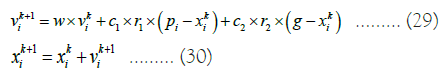
Random optimization using PSO
PSO is an effective optimization method when dealing with optimization based on non-smooth simulation. In addition, as a zero order optimization method, the particle swarm optimization algorithm does not require a derivative regarding free parameters. In addition, PSO is a random method that allows us to find the global optimal value among all local optima.
Step1: Initialize the position and velocity of the particle swarm.
Randomly generate a set of initial positions and velocities of particles, each representing the design parameters of a heliostat.
Set the fitness function of each particle as the average output thermal power per unit area.
Step2: For each particle, use Monte Carlo algorithm to simulate the optical efficiency of the heliostat and calculate the average output thermal power per unit area.
At the position of each particle, Monte Carlo algorithm is used for optical efficiency simulation.
Estimate the average output thermal power per unit area through random sampling.
Step3: Update the speed and position of particles.
Update the velocity and position of each particle based on individual and group experience. By adjusting the speed and position, particles are moved towards a direction with higher fitness.
Step4: Repeat steps 2 and 3 until the stop condition is reached. Repeat steps 2 and 3 until the stop condition is met. The stopping condition can be reaching the maximum number of iterations or meeting the convergence condition.
Step5: Output optimal solution. After the stop condition is met, select the particle with the maximum average output thermal power per unit area as the optimal solution.
Output the optimal solution, which is the design parameter of the heliostat with the maximum average output thermal power per unit area (Figure 15).

Figure 15: The result graph obtained by solving the convergence condition after 12 iterations.
The two numbers r1 and r2 are uniformly sampled random numbers (0,1) and are used to influence the randomness of the algorithm. The weight inertia w is used to control the convergence behaviour of PSO. The coefficients c1 and c2 control how far the particle moves in the search space in a single iteration. c1 directs the individual behaviour of the particle, while c2 directs its social behaviour. In addition, a speed clamping vmax definer with maximum speed gain is set |vmax|=k × (xmax-xmin)/2. When k is used, the user-supplied speed clamping factor is fixed at 0.1.
Each heliostat generated by PSO (i.e., each generated SPT system geometry described by a set of parameters) is evaluated using a direct model. The simulation results are used to determine particle performance as they are input values for the objective function.
Radial grid method for optimizing heliostat models
The heliostat is an important device for the energy source of the entire system, and its comprehensive efficiency determines the total amount of energy sources in the entire system. Therefore, the layout of the heliostat in the mirror field is particularly important. This article uses the radial grid method to design the heliostat field.
The core idea of the radial grid method is to draw circles of different sizes with the centre of the bottom surface of the absorption tower as the centre, so that the centres of the heliostats are distributed on these circles. The positions of the centres of the heliostats on adjacent circles are staggered from each other, not on the same straight line, but form a staggered pattern, as shown in the following, Figure 16, where is the radial spacing of △R, and △Z is the distance between the centres of adjacent heliostats on the same circle [7].

Figure 16: Schematic diagram of the physical model for the misaligned
arrangement of heliostats. Note:  centres of heliostats.
Due to the need to reserve a certain safety distance between two heliostats, the number of heliostats on the latter ring is the same as that on the previous ring, so the heliostats on each ring in the same layout area have the same circumferential angle. The heliostats on the front and rear rings are arranged in a staggered manner. To quantitatively represent the position relationship between the heliostats and the heat absorption tower, a calculation formula is introduced:
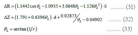
In the above formula, h is the height of the mirror surface, d is the width of the mirror surface, θL is the height angle of the collector relative to the heliostat, and r is the distance between the heliostat and the absorption tower in units of distance from the centre of the collector to the centre point of the heliostat (Figure 17).

Figure 17: Initial arrangement of heliostats.
Summary of solution results for research 2
Explanation for selecting the coordinates of the absorption tower position: In the research 1, it is solved that when the sun is located between the equator and the Tropic of Cancer, the shadow shading loss caused by the projection of the absorption tower is relatively small due to the mirror field being located at 39.4° N, and there is even no loss between some months. However, when the sun is located between the equator and the Tropic of Cancer, the sun is located south of the tower, and the shadow shading loss caused by the tower body projection is relatively large, and it cannot be ignored. The title clearly stipulates that the construction scope of the heliostat field is a circular area with a radius of 350 m, and no heliostats are installed within a range of 100 m around the tower body [8,9].
The coordinate position of the tower is set at (0, -200), and the horizontal coordinate range of the heliostats that can be used for construction is (-300, -350) and (-100, 350), which can effectively reduce the shadow blocking loss caused by the tower body projection. The parameter values for effectively optimizing shadow occlusion efficiency (Tables 7-9).
| Date | Average Optical efficiency | Average cosine efficiency | Average Shadow Occlusion Efficiency | Average truncation efficiency | Average output thermal power per unit area mirror (kw/m2) |
|---|---|---|---|---|---|
| January 21st | 0.6283 | 0.8415 | 0.8282 | 0.9972 | 0.611 |
| February 21st | 0.6182 | 0.8539 | 0.8119 | 0.9904 | 0.5927 |
| March 21st | 0.6081 | 0.8401 | 0.8113 | 0.999 | 0.6089 |
| April 21st | 0.6083 | 0.8449 | 0.827 | 0.9846 | 0.602 |
| May 21st | 0.611 | 0.8612 | 0.8352 | 0.9977 | 0.613 |
| June 21st | 0.6254 | 0.8528 | 0.8403 | 0.9884 | 0.5909 |
| July 21st | 0.6109 | 0.8517 | 0.8138 | 0.984 | 0.5997 |
| August 21st | 0.6248 | 0.8642 | 0.8283 | 0.9877 | 0.5916 |
| September 21st | 0.6107 | 0.8427 | 0.8249 | 0.9899 | 0.6122 |
| October 21st | 0.6276 | 8587 | 0.8099 | 0.9959 | 0.5892 |
| November 21st | 0.6133 | 0.8586 | 0.8206 | 0.9813 | 0.6077 |
| December 21st | 0.6095 | 0.8459 | 0.8148 | 0.9871 | 0.6087 |
Table 7: Research 2-average optical efficiency and output power on the 21st day.
| Average optical efficiency | Average cosine efficiency | Average Shadow Occlusion efficiency | Average Truncation efficiency | Annual average thermal power output (MW) | Annual average output of mirror surface per unit area Thermal power (kw/m2) |
|---|---|---|---|---|---|
| 0.6163 | 0.8521 | 0.8222 | 0.9903 | 62.18 | 0.6023 |
Table 8: Annual average optical efficiency and output power table.
| Absorption tower position coordinates | Heliostat size (W × H) | Heliostat mounting height (m) | Total number of heliostats | Total heliostat area (m2) |
|---|---|---|---|---|
| (0, -200) | 3.5 × 3.5 | 2 | 8440 | 103390 |
Table 9: Research 2-design parameter table.
Establishment and solution of research 3 model
This research is based on research 2, removing the constraint that the size parameters and installation height of each heliostat are the same, while keeping everything else unchanged. To solve this research, the area where the heliostat is installed can be divided into a circular area of 3 to 6.
The size and installation height of heliostats in the same area are the same, while the size and installation height of heliostats in different rings are different. By bringing it into the established optimization model, the optimal design parameters can be solved. The detailed data can be found in the supporting materials of research three. The following Tables 10-14, summarizes the data of the heliostat in the closest ring to the heat absorption tower.
| Date | Average Optical efficiency | Average cosine efficiency | Average shadow occlusion efficiency | Average truncation efficiency | Average output thermal power per unit area mirror (kw/m2) |
|---|---|---|---|---|---|
| January 21st | 0.1485 | 0.6199 | 0.8735 | 0.2584 | 0.1227 |
| February 21st | 0.1516 | 0.6404 | 0.8957 | 0.2480 | 0.1399 |
| March 21st | 0.1549 | 0.6611 | 0.8998 | 0.2462 | 0.2538 |
| April 21st | 0.1585 | 0.6793 | 0.8999 | 0.2473 | 0.1646 |
| May 21st | 0.1611 | 0.6893 | 0.9 | 0.2488 | 0.1705 |
| June 21st | 0.1619 | 0.6923 | 0.9 | 0.2494 | 0.1724 |
| July 21st | 0.1511 | 0.6892 | 0.9 | 0.2488 | 0.1705 |
| August 21st | 0.1583 | 0.6786 | 0.8999 | 0.2472 | 0.1642 |
| September 21st | 0.1548 | 0.6601 | 0.8997 | 0.2462 | 0.1531 |
| October 21st | 0.1512 | 0.6378 | 0.8941 | 0.2487 | 0.1380 |
| November 21st | 0.1483 | 0.6182 | 0.8710 | 0.2597 | 0.1209 |
| December 21st | 0.1471 | 0.6111 | 0.8561 | 0.2672 | 0.1133 |
Table 10: Average optical efficiency and output power on 21 days of each month.
| Average optical efficiency | Average cosine efficiency | Average Shadow Occlusion efficiency | Average Truncation efficiency | Annual average thermal power output (MW) | Annual average output of mirror surface per unit area Thermal power (kw/m2) |
|---|---|---|---|---|---|
| 0.1548 | 0.6564 | 0.8908 | 0.2513 | 9.878 | 0.1487 |
Table 11: Table of three-year average optical efficiency and output power.
| Absorption tower position coordinates | Heliostat size (W × H) | Heliostat mounting height (m) | Total number of heliostats | Total heliostat area (m2) |
|---|---|---|---|---|
| (0,-200) | 4 × 4 | 3 | 1580 | 25280 |
Table 12: Design parameters.
| Average optical efficiency | Average cosine efficiency | Average Shadow Occlusion efficiency | Average Truncation efficiency | Annual average thermal power output (MW) | Annual average output of mirror surface per unit area Thermal power (kw/m2) |
|---|---|---|---|---|---|
| 0.6263 | 0.8154 | 0.8398 | 0.9973 | 62.256 | 0.6187 |
Table 13: Total annual average optical efficiency and output power table.
| Absorption tower position coordinates | Heliostat size (W × H) | Heliostat mounting height (m) | Total number of heliostats | Total heliostat area (m2) |
|---|---|---|---|---|
| (0, -200) | 7140 | 100638.4354 |
Table 14: General design parameters.
Model verification
Stability test: This article tests the stability of the model by floating the relevant parameter values up and down. When calculating the optical efficiency, it involves five parameters: Shadow occlusion efficiency ηsb, cosine efficiency ηcos, atmospheric transmittance ηat, collector truncation efficiency ηtrunc, and mirror reflectance ηref. The data for each parameter from January to December are fluctuated by 5% up and 10% up and down, respectively. Then use the plot function of MATLAB software to draw a visualized line graph, and analyse the stability of the model based on the line graph.
From Figure 18, it can be seen that by floating the values of the relevant parameters up and down by 5% and up and down by 10%, the final calculated results all revolve around a single value, but the range of fluctuations is not large and has good stability.

Figure 18: Data visualization. Note:  Original figure,
  lower 10%,
  lower 5%, up-regulation 5%, up-regulation 10%.
Therefore, it can be inferred that the model has good stability.
Sensitivity test: In the sensitivity analysis of the model, we can consider increasing the number of heliostats to construct a larger circular field to meet higher output thermal power requirements. Assuming we increase the number of heliostats to over 1745, we can calculate the area of the new heliostat field and the output thermal power.
According to the result of the first research, when the number of heliostats is 1745, the area of the heliostat field is S=π × 350 × 350=3926500 m2.
Assuming we increase the number of heliostats to N, i.e. N>1745, the area of the heliostat field can be expressed as S=π × 350 × 350 × N.
According to the requirements of the research, when the rated annual average output thermal power of the heliostat field reaches 60 MW, the following equation can be listed:
60000 kW=Area × reflectivity × Sun incidence angle × Solar altitude angle × Atmospheric transparency
Among them, the solar incidence angle, solar altitude angle, and atmospheric transparency are known constants. By substituting the area into the equation, we can obtain:
60,000 kW=π × 350 × 350 × N × reflectance × (sin(Angle of incidence)) × (cos(Angle of incidence))2 × (sin(Altitude Angle)) × (cos(Altitude Angle))2 × (sin(Atmospheric transparency))
By adjusting the number N of heliostats, different output thermal power requirements can be met. For example, if you want to output a thermal power of 80 MW, you can set N to around 1800. It should be noted that increasing the number of heliostats will increase the complexity and computational complexity of the system. Therefore, in practical applications, it is necessary to comprehensively consider the actual situation for reasonable design.
Advantages of the model
When solving research 2, the Monte Carlo algorithm and PSO algorithm are combined to optimize the optical efficiency of the heliostat, while also fully considering the optimization of heliostat design parameters. The Monte Carlo algorithm can estimate the average output thermal power per unit area through random sampling, which can more accurately simulate the optical efficiency of a heliostat. PSO algorithm has good global search ability and can search for the optimal solution by learning the experiences of individuals and populations. This algorithm can comprehensively consider optical efficiency and thermal power output when designing heliostats.
Disadvantages of the model
When the Monte Carlo algorithm has high computational complexity, it requires a large amount of random sampling to estimate the value of the objective function, which can lead to a longer computational time.
PSO algorithm is sensitive to the selection of initial parameters, and selecting different initial parameters may lead to different optimal solutions. At the same time, the algorithm may only be able to find local optimal solutions, but cannot find global optimal solutions. Moreover, the algorithm relies heavily on the search space for the parameter design of the heliostat, meaning that the size of the search space may have an impact on the algorithm's performance.
Model improvement
Because it is time-consuming to reorient the heliostat on each date, this article chooses to reduce the number of sampling dates. However, due to the requirements for estimation accuracy, this article adopts a systematic sampling method, which involves sampling several rays per date.
This article uses computer graphics technology to optimize photon tracking algorithms for optimization. Optimize photon tracking algorithms through computer graphics technology to reduce computational time during heliostat reorientation. Each heliostat is enclosed in an expanded cubic bounding box, which includes all possible positions of the heliostat when tracking the sun.
This algorithm model can be combined with other optimization algorithms, such as genetic algorithm and differential evolution algorithm, to construct a hybrid optimization algorithm. By combining different optimization methods, the advantages of various algorithms can be combined to improve global search ability and convergence speed.
This algorithm can consider uncertainty and robustness. In practical applications, there may be various uncertain factors, such as fluctuations in material parameters, changes in environmental conditions, etc. Therefore, we can consider introducing uncertain factors into the model and solve the robust optimal solution through robust optimization methods. By considering uncertainty and robustness, the design scheme can have better stability and reliability.
Promotion of the model
In practical life, this model can be applied to the following fields for promotion:
Design of solar power generation systems: This model can be applied to optimize the design of solar power generation systems. By optimizing the design parameters of components such as solar panels, inverters, and energy storage systems, the energy conversion efficiency and output power of solar power generation systems can be improved.
Optical device design: In addition to heliostats, this model can be applied to optimize the design of other optical devices, such as optical lenses, fibres, optical sensors, etc. By optimizing the design parameters of optical devices, their optical performance, transmission efficiency, and sensitivity can be improved.
Photovoltaic power plant layout optimization: This model can be applied to the layout optimization of photovoltaic power plants. By optimizing the layout and orientation of photovoltaic panels, the total power generation of photovoltaic power plants can be maximized, and the economic benefits and energy utilization efficiency of photovoltaic power plants can be improved.
Optical communication network design: This model can be applied to optimize the design of optical communication networks. By optimizing design parameters such as fibre routing and placement of optical amplifiers, the transmission rate, signal quality, and coverage of optical communication networks can be improved.
By applying this model to various fields in real life, design solutions can be optimized to improve energy utilization efficiency, transmission efficiency, and system performance, thereby achieving the goals of sustainable development and energy conservation and emission reduction.
As for research objective 1, the average annual optical efficiency of heliostat field is 0.4512, the average output thermal power is 27.5713 MW, and the average annual output thermal power per unit mirror area is 0.4401 kw/m2.
As for research objective 2, the optimal design parameters are obtained as follows: the position coordinate of the absorption tower is (0, -200), the size of the heliostat is 3.5 m × 3.5 m, the installation height is 2 m, the total number of surfaces of the heliostat is 8440, and the total area is 103390 m2.
As for research objective 3, the optimal design parameters are obtained as follows: The helioscope installation area is divided into four ring areas. The size and installation height of helioscopes in the same area are the same, while the size and installation height of helioscopes in different rings are different. The position coordinates of the absorption tower are (0,-200), and the size of the helioscope ranges from 4 m × 4 m to 3.5 m × 3.5 m from near too far. The installation height from near to far is 2.1 m~6 m, the total number of heliostat is 7147, and the total area is 104690.89 m2.
This work was supported by the Philosophical and Social Sciences Research Project of Hubei Education Department (19Y049), and the Staring Research Foundation for the Ph.D. of Hubei University of Technology (BSQD2019054), Hubei Province, China.
We have no conflict of interests to disclose and the manuscript has been read and approved by all named authors.
Citation: Zhao B, Jiang X, Wu Y (2023) Optimization Design of Heliostat Field Based on Monte Carlo and PSO Algorithms. J Phys Chem Biophys. 13:364.
Received: 03-Oct-2023, Manuscript No. JPCB-23-27280; Editor assigned: 05-Oct-2023, Pre QC No. JPCB-23-27280 (PQ); Reviewed: 19-Oct-2023, QC No. JPCB-23-27280; Revised: 26-Oct-2023, Manuscript No. JPCB-23-27280 (R); Published: 02-Nov-2023 , DOI: 10.35248/2161-0398.23.13.364
Copyright: © 2023 Zhao B, et al. This is an open-access article distributed under the terms of the Creative Commons Attribution License, which permits unrestricted use, distribution, and reproduction in any medium, provided the original author and source are credited.