Journal of Pollution Effects & Control
Open Access
ISSN: 2375-4397
ISSN: 2375-4397
Research Article - (2016) Volume 4, Issue 1
In Mandi-Gobindgarh, Punjab, India, open crop residue burning is one of the major sources of air pollution in the area besides pollutions from industries, vehicles, etc. In this paper, the impact of open crop residue burning on the concentrations of particulate matters (PM10 and PM2.5) in ambient air for paddy and wheat crops were monitored at five different locations during year 2012-2013. The air quality data for PM10 and PM2.5 were subjected to non-linear regression analysis for both paddy and wheat crop seasons. The regression models for PM10 are best described by the power functions, while for PM2.5 by the exponential functions with R2 values higher than 0.99. These models may prove useful tool in estimation of the PM10 and PM2.5 concentrations in ambient air for the areas where stubble burning is practiced by farmers.
Keywords: Ambient air quality; Crop residue burning; PM10; PM2.5; Non-linear regression model
Burning of crop residue has been an agricultural practice, especially in the developing countries like India, as it is one of the cheapest ways of disposal, less time consuming and less laborious to prepare the land for further farming. It deteriorates the ambient air quality by producing large amounts of particulate matters and gases into the atmosphere. The ambient air quality of Mandi-Gobindgarh, Punjab, India has been degraded a lot during the last few years due to extensive industrialization as well as crop residue burning. The Cumulative Environmental Pollution Index (CEPI) for Mandi-Gobindgarh with respect to air was calculated to be 62 [1]. Due to this reason, Mandi- Gobindgarh is declared as critically polluted area [2]. Apart from the industries and vehicular emissions, crop residue burning in agricultural fields is one of the main reasons for the deterioration of the ambient air quality of Mandi-Gobindgarh area.
To prepare the fields for the subsequent crop to be sown, crop residue burning is done by the farmers for clearing the land from stubble and weeds. Biomass burning is one of the major sources of gaseous and particulate emissions in to the atmosphere. Therefore, monitoring of particulate matters especially PM10 and PM2.5 in the ambient air is necessary as they causes severe adverse health effects on human beings residing in such area.
Limited studies on gaseous and particulate emissions from open burning of crop residue, especially in an industrial area, have been reported. In the survey by Gao et al., [3], on an average, only 6.6% of the crop residue is burned in the fields and 36.6% of the crop residue is returned to the soil directly. Ground-based ambient air monitoring at five different locations in and around Patiala city was conducted in order to determine the impact of open burning of rice crop residues on SPM, SO2 and NO2 concentrations in the ambient air. Substantially higher concentrations of PM10 and PM2.5 were reported by Singh et al. [4] at the commercial areas as compared to the other sampling sites. Gupta et al. [5] studied the type as well as amount of air pollutants in industrial town of Mandi-Gobindgarh as well as surrounding areas and reported that the cause of urban air pollution is mainly due to presence of excessive suspended particulate matters, whereas, in rural areas, air is polluted by particulate matters as well as CO2 and NOx from stubble burning. Demuzere and Lipzig [6] used a multiple linear regression technique combined with the automated Lamb weather classification to make projections for the future air quality levels. Akpinar et al. [7], studied the relationship between monitored air pollutant concentrations and meteorological factors using linear and non-linear regression models and observed that there exist a moderate and weak correlation between the air pollutant concentrations and the meteorological factors. The present study aims to develop non-linear regression models to predict the PM10 and PM2.5 concentrations in the ambient air due to open biomass burning based on the experimental study conducted in Mandi-Gobindgarh district in Punjab, India.
Study area
Mandi-Gobindgarh is a town located in Fatehgarh Sahib District in the state of Punjab, India and is also known as ‘Steel Town of India’ as various steel manufacturing industries is operating in this town. The town is located on National Highway-I and spread over an area of 10.64 Sq. kms with population of 55,416 as per 2001 census records. Geographically, Mandi-Gobindgarh is situated in between north latitude 30°-37’-30”and 30°-42’-30” and east longitude 76-15’ and 76°- 20’. There are 510 coal/oil based industries (404 in Mandi-Gobindgarh and 106 in Khanna area) causing air pollution in the area besides the fugitive emissions [1]. On the basis of land use, demography and industrial clusters, five sampling sites were selected for the study. Eight industrial clusters have been identified within the jurisdiction of critically polluted area of Mandi-Gobindgarh and Khanna area (PPCB, 2010)1. The site location and its classification are presented below in Table 1.
| Site No. | Site classification | Site location | Site description | Percent area covered |
| 1 | Agricultural Site | 20 kms South-East of Mandi-GobindgarhLatitude: 30°34'23.16"N Longitude:76°21'47.43"E | It is a broad open area with no side buildings with no industries | 100%agricultural area |
| 2 | Mixed-land use site(I) | 2 kms North of AmlohChowk Latitude:30°38'45.86"N Longitude:76°16'1.97"E | Partially industrialized area, major proportion is covered by agriculture | 30% industrial area and 70% agricultural area |
| 3 | Mixed-land use site(II) | National highway (NH1) Latitude:30°39'5.91"N Longitude:76°19'24.53"E | Broad open area with no side buildings with high vehicular pollution | 60% area covered by highway and 20% agricultural and industrial area |
| 4 | Mixed-land use site(III) | Guru kinagri, south-east on GT road from Mandi-Gobindgarh bus stand Latitude:30°40'18.77"N Longitude:76°17'38.29"E | Semi- urban site, having mixed land use comprising of industrial, residential and agricultural area | 80% industrial and 20% agricultural area |
| 5 | Industrial site | Industrial focal point, 2 kms South-west from MandiGobindgarh bus standLatitude: 30°38'34.97"N Longitude:76°18'27.03"E | Area is less populated as land use of the area is totally industrial | 100% Industrial area |
Table 1: Site location and classification.
Measurement of PM10 and PM2.5
The weather monitoring station used in this study was Watch Dog of Spectrum Series 2000. The Watch Dog weather station is a multifunction device to detect as well as to store seven parameters including wind speed, wind direction, temperature, relative humidity, dew point, pressure and solar radiations using different sensors for each parameter. For measurement of PM10 and PM2.5 in ambient air, Ambient Fine Dust Sampler (Model no. IPMFDS-
2.5 μ/10 μ of INSTRUMEX) was used and it conforms to the USEPA, USA and CPCB, India norms. For sampling of PM10, Whatman 1820- 047 filter paper having 47 mm diameter, while for sampling of PM2.5, Whatman 7582-004 filter paper having 37 mm diameter and PTFE filters having diameter 46.2 mm were used [8,9].
Sampling of PM10 and PM2.5 was carried out for rice and wheat harvesting periods starting from September 2012 to May 2013, at all the five selected sites. The total time period of monitoring has been categorized as pre-harvesting period (September, 2012 for rice and February to March, 2013 for wheat); harvesting period (October- November, 2012 for rice and April, 2013 for wheat) and post-harvesting period (December, 2012 to January, 2013 for rice and May, 2013 for wheat). Each new blank filter paper was conditioned over dried silica gel, prior to use, in a desiccator for 24 hrs and weighed at room temperature (25°C). Pre-inspected and weighed new blank filters were placed into the sampling device for continuous sampling. After 24 h of sampling, an exposed filter paper was reweighed; data were retrieved from the instrument to get initial and final flow rate for each sample and the concentrations of PM10 and PM2.5 were calculated as follows. The volume of air sampled was calculated using following equation.
Va =(F1+F2) × T/2 (1)
Where, Va is the volume of air sampled in m3, F1 and F2 are the measured flow rates before and after sampling in LPM and T is time of sampling in minutes.
PM10 concentration was calculated by the following expression,
PM10 = (Wf-Wi) × 1000/Va (2)
Where, PM10 is total mass concentration of PM10 collected during the sampling period in μg/m3, Wf and Wi are the final and initial mass of glass fiber filter paper in mg, Va is the total air volume sampled in m3.
PM2.5 concentration was calculated by:
PM2.5=(Wf ‘-Wi’) × 1000/Va (3)
Where, PM2.5 is total mass concentration of PM2.5 collected during the sampling period in μg/m3, Wf’ and Wi’ are the final and initial mass of PTFE filter paper in mg.
Using Eq’s (1), (2) and (3) PM10 and PM2.5 concentrations were calculated for all the sampling sites during three sampling periods viz. pre-harvesting, during harvesting and post-harvesting. Tables 2 and 3 shows the experimental concentration of PM10 and PM2.5 for paddy and wheat crops respectively.
| Site No. | Sample No. | PM10 experimental conc. for three sampling periods for paddy crop | PM10 experimental conc. for three sampling periods for wheat crop | ||||
| Pre-harvesting | During harvesting | Post-harvesting | Pre-harvesting | During harvesting | Post-harvesting | ||
| 1 | 1 | 228.2 | 376.4 | 336 | 285.1 | 458.5 | 420.5 |
| 2 | 260.4 | 432.9 | 368.6 | 316.5 | 495.8 | 447.8 | |
| 2 | 3 | 328.4 | 490.8 | 398.7 | 355.8 | 530.6 | 473.4 |
| 4 | 344.2 | 502.9 | 429.2 | 375.2 | 548.7 | 487.1 | |
| 3 | 5 | 380.1 | 525.6 | 442.6 | 400.3 | 559.1 | 499.6 |
| 6 | 400 | 539.7 | 458.9 | 419.1 | 566.2 | 508.8 | |
| 4 | 7 | 425.3 | 557.7 | 480.2 | 438.7 | 587.4 | 522.3 |
| 8 | 439.2 | 569.9 | 492.1 | 449.5 | 595.2 | 528.6 | |
| 5 | 9 | 461.5 | 583.9 | 508.2 | 465.5 | 600.1 | 542.2 |
| 10 | 473.3 | 592.3 | 518.4 | 480.6 | 617.2 | 551.4 | |
Table 2: Experimental concentrations of PM10.
Non-Linear regression analysis
Since high concentrations of particulate matters affect the public health, much attention is required to be paid towards the improvement of the accuracy of short-term deterministic and statistical models and the development of robust long-term air-quality prediction models.
Modeling of PM10 and PM2.5 concentrations due to burning of crop residues are not explored well in the literature. Due to this reason, a non-linear regression model for assessment of
PM10 and PM2.5 concentrations have been developed in the present work, to observe the effects of crop residue burning prior, during and after harvesting periods. Regression analysis is attempted to find the relationship between the variables and to obtain the best regression equation for the accurate predictions of PM10 and PM2.5 concentrations. The goodness of fit is ascertained by the coefficient of determination (R2). In addition to R2, the various statistical parameters such as; mean, root mean square error (RMSE), Marquardt’s percent standard deviation (MPSD), standard error (SE) and sum of square error (SSE) were also used to determine the accuracy of the best fitted regression models [10].PM10 and PM2.5 concentrations have been developed in the present work, to observe the effects of crop residue burning prior, during and after harvesting periods. Regression analysis is attempted to find the relationship between the variables and to obtain the best regression equation for the accurate predictions of PM10 and PM2.5 concentrations. The goodness of fit is ascertained by the coefficient of determination (R2). In addition to R2, the various statistical parameters such as; mean, root mean square error (RMSE), Marquardt’s percent standard deviation (MPSD), standard error (SE) and sum of square error (SSE) were also used to determine the accuracy of the best fitted regression models [10].
Non-linear regression analysis of PM10 in ambient air
The experimental concentrations of PM10 as presented in Table 2 are plotted against sample number (Time) for all the three sampling periods. Figure 1a-1c show the variation of PM10 concentration for paddy and wheat crops respectively during pre-harvesting, harvesting and post-harvesting periods. From Figures 1a-1c, it is evident that the variation of PM10 concentration is well described by a non-linear power function with R2 values more than 0.99 in all the three cases. Thus power function appears to be suitable non-linear regression model for prediction of PM10 concentration for paddy and wheat crops for pre-, during and post-harvesting periods. The predicted and experimental PM10 concentrations along with percentage error are shown in Table 4 for both paddy and wheat crops, which are in close agreement with each other.
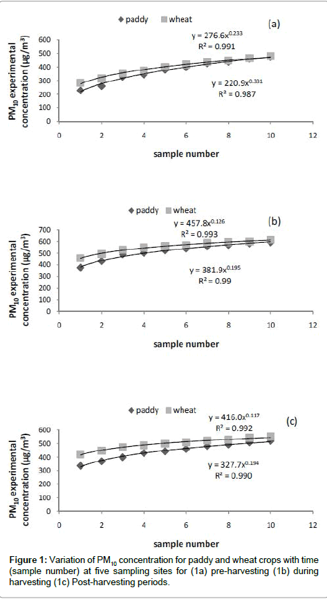
Figure 1: Variation of PM10 concentration for paddy and wheat crops with time (sample number) at five sampling sites for (1a) pre-harvesting (1b) during harvesting (1c) Post-harvesting periods.
| Site No. | Sample No. | Paddy | Wheat | ||||||||||||||||
| Pre-harvesting | During harvesting | Post-harvesting | Pre-harvesting | During harvesting | Post-harvesting | ||||||||||||||
| Experimental conc. | Predicted conc. | % error | Experimental conc. | Predicted conc. | % error | Experimental conc. | Predicted conc. | % error | Experimental conc. | Predicted conc. | % error | Experimental conc. | Predicted conc. | % error | Experimental conc. | Predicted conc. | % error | ||
| 1 | 1 | 228.2 | 220.9 | 3.2 | 376.4 | 381.9 | -1.5 | 336 | 327.7 | 2.5 | 285.1 | 276.6 | 3 | 458.5 | 457.8 | 0.1 | 420.5 | 416.1 | 1.1 |
| 2 | 260.4 | 278.1 | -6.8 | 432.9 | 437.2 | -0.9 | 368.6 | 374.9 | -1.7 | 316.5 | 325.2 | -2.8 | 495.8 | 499.6 | -0.8 | 447.8 | 451.2 | -0.8 | |
| 2 | 3 | 328.4 | 318.1 | 3.1 | 490.8 | 473.1 | 3.6 | 398.7 | 405.6 | -1.7 | 355.8 | 357.5 | -0.5 | 530.6 | 525.8 | 0.9 | 473.4 | 473.2 | 0.04 |
| 4 | 344.2 | 349.9 | -1.7 | 502.9 | 500.4 | 0.5 | 429.2 | 428.9 | 0.1 | 375.2 | 382.3 | -1.9 | 548.7 | 545.2 | 0.6 | 487.1 | 489.4 | -0.5 | |
| 3 | 5 | 380.1 | 376.9 | 0.8 | 525.6 | 522.7 | 0.6 | 442.6 | 447.9 | -1.2 | 400.3 | 402.7 | -0.6 | 559.1 | 560.7 | -0.3 | 499.6 | 502.4 | -0.6 |
| 6 | 400 | 400.4 | 0.1 | 539.7 | 541.6 | 0.4 | 458.9 | 463.9 | -1.1 | 419.1 | 420.2 | -0.3 | 566.2 | 573.8 | -1.3 | 508.8 | 513.2 | -0.9 | |
| 4 | 7 | 425.3 | 421.4 | 0.9 | 557.7 | 558.1 | -0.1 | 480.2 | 478.1 | 0.4 | 438.7 | 435.6 | 0.7 | 587.4 | 585 | 0.4 | 522.3 | 522.5 | -0.04 |
| 8 | 439.2 | 440.5 | -0.3 | 569.9 | 572.9 | -0.5 | 492.1 | 490.6 | 0.3 | 449.5 | 449.4 | 0.02 | 595.2 | 594.9 | 0.04 | 528.6 | 530.8 | -0.4 | |
| 5 | 9 | 461.5 | 458 | 0.7 | 583.9 | 586.2 | -0.4 | 508.2 | 501.9 | 1.2 | 465.5 | 461.9 | 0.8 | 600.1 | 603.9 | -0.6 | 542.2 | 538.1 | 0.7 |
| 10 | 473.3 | 474.3 | -0.2 | 592.3 | 598.3 | -1 | 518.4 | 512.3 | 1.2 | 480.6 | 473.4 | 1.5 | 617.2 | 611.9 | 0.9 | 551.4 | 544.8 | 1.2 | |
Table 4: Experimental and predicted PM10 concentration with percent error.
A comparison of the PM10 concentrations between predicted and experimental values for paddy and wheat crops are shown in Figure 2a-2c and Figure 3a-3c respectively. From Figure 2a-2c and Figure 3a-3c, it is evident that predictions of PM10 concentrations using developed non-linear regression models, are in close agreement with experimental PM10 concentrations within the maximum error bands of ± 6.8%, which is within acceptable limit..
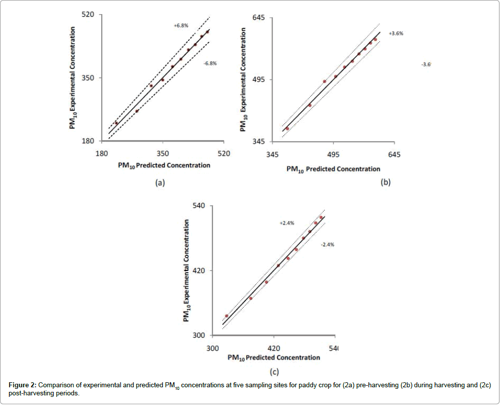
Figure 2: Comparison of experimental and predicted PM10 concentrations at five sampling sites for paddy crop for (2a) pre-harvesting (2b) during harvesting and (2c) post-harvesting periods.
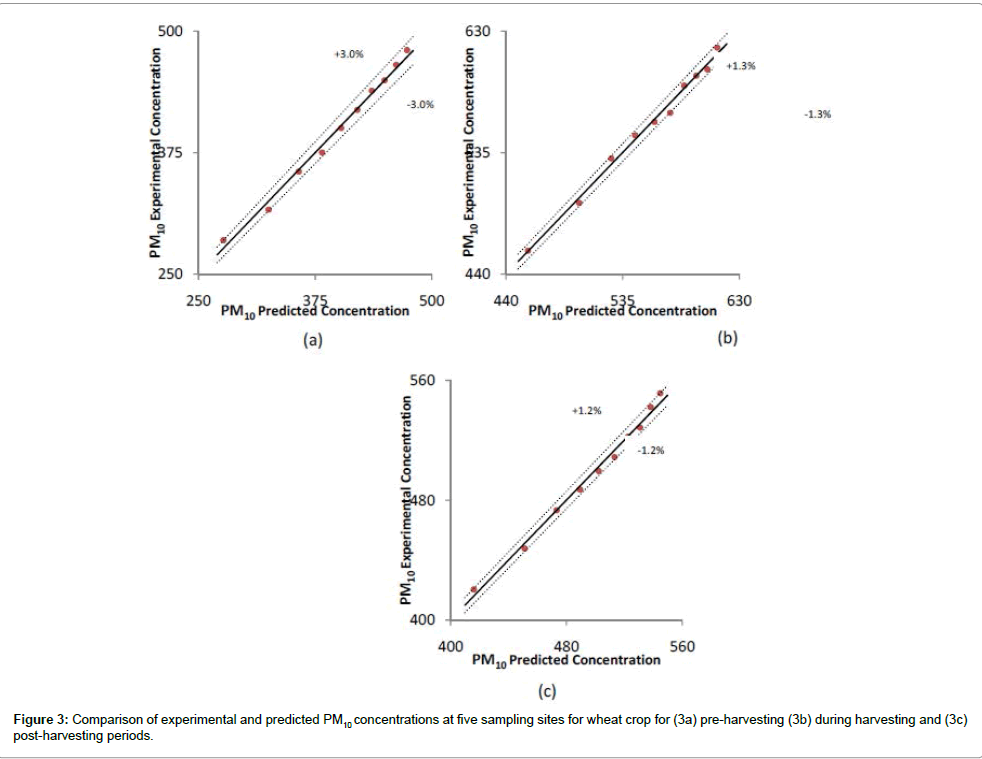
Figure 3: Comparison of experimental and predicted PM10 concentrations at five sampling sites for wheat crop for (3a) pre-harvesting (3b) during harvesting and (3c) post-harvesting periods.
The statistical parameters (R2, Mean, MPSD, RMSE, SSE and SE) using predicted values are determined using their basic definitions and expressions available in literature [10] are presented in Tables 5 and 6 for paddy and wheat crops respectively. From these tables it is evident that RMSE values are quite low and hence, predictions of PM10 concentrations are in close agreement with the experimental PM10 concentrations.
| PM10 concentration for paddy crop | |||||||
| Sampling Periods | Statistical parameters | ||||||
| Regression Equation | R2 | Mean | MPSD | RMSE | SSE | SE | |
| Pre-Harvesting | y=220.95x0.3318 | 0.987 | 373.872 | 0.0298 | 7.38 | 0.035 | 8.225 |
| During harvesting | y=381.9x0.195 | 0.99 | 517.248 | 0.0151 | 6.552 | 0.001 | 7.255 |
| Post-Harvesting | y=327.7x0.1941 | 0.99 | 443.201 | 0.0149 | 5.398 | 0.008 | 5.945 |
Table 5: Regression equation and statistical parameters for PM10 concentration for paddy crop.
| PM10 concentration for wheat crop | |||||||
| Sampling Periods | Statistical parameters | ||||||
| Regression Equation | R2 | Mean | MPSD | RMSE | SSE | SE | |
| Pre-Harvesting | y=276.67x0.2333 | 0.991 | 398.51 | 0.017 | 5.306 | 0.013 | 5.809 |
| During harvesting | y = 457.82x0.126 | 0.994 | 555.87 | 0.008 | 3.975 | 0.0001 | 4.444 |
| Post-Harvesting | y = 416.07x0.1171 | 0.992 | 498.18 | 0.008 | 3.58 | 0.0001 | 3.986 |
Table 6: Regression equation and statistical parameters for PM10 concentration for wheat crop.
Non-linear regression analysis of PM2.5 in ambient air
The experimental concentrations of PM2.5 as presented in table 3 are plotted against sample number (Time) for all the three sampling periods. Figures 4a-4c show the variation of PM2.5 concentration for paddy and wheat crops respectively during pre-harvesting, harvesting and post-harvesting periods. Using these regression equations as presented within these figures, the predicted values were calculated. Table 7 shows the experimental and predicted PM2.5 concentrations along with percent error in predictions. The maximum errors in predictions are limited to 4.7%. From Figure 4a-4c, it is evident that the variation of PM2.5 concentration is well described by a non-linear exponential function with R2 values more than 0.99 in all the three cases. Thus exponential functions so developed are suitable non-linear regression model for prediction of PM2.5 concentrations for both paddy and wheat crops for pre-, during and post-harvesting periods.
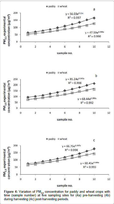
Figure 4: Variation of PM2.5 concentration for paddy and wheat crops with time (sample number) at five sampling sites for (4a) pre-harvesting (4b) during harvesting (4c) post-harvesting periods.
| Site No. | Sample No. | Paddy | Wheat | ||||||||||||||||
| Pre-harvesting | During harvesting | Post-harvesting | Pre-harvesting | During harvesting | Post-harvesting | ||||||||||||||
| Experimental conc. | Predicted conc. | % error | Experimental conc. | Predicted conc. | % error | Experimental conc. | Predicted conc. | % error | Experimental conc. | Predicted conc. | % error | Experimental conc. | Predicted conc. | % error | Experimental conc. | Predicted conc. | % error | ||
| 1 | 1 | 63.54 | 62.5 | 1.6 | 94.1 | 93.6 | 0.6 | 75.2 | 73.6 | 2.2 | 50.2 | 52.5 | -4.7 | 73.2 | 74.9 | -2.4 | 65.4 | 66.1 | -1.1 |
| 2 | 69.7 | 69.8 | -0.2 | 102 | 102.7 | -0.7 | 79.9 | 81.1 | -1.5 | 56.5 | 58 | -2.7 | 80.1 | 82.1 | -2.5 | 70.2 | 72.3 | -3 | |
| 2 | 3 | 75.8 | 77.9 | -2.8 | 110.5 | 112.7 | -2 | 90 | 89.3 | 0.7 | 65.8 | 64.1 | 2.7 | 90.3 | 89.9 | 0.4 | 80.3 | 79 | 1.6 |
| 4 | 85.6 | 86.9 | -1.6 | 124.5 | 123.8 | 0.6 | 97.1 | 98.5 | -1.4 | 73.2 | 70.7 | 3.4 | 99.7 | 98.5 | 1.3 | 87.2 | 86.4 | 0.9 | |
| 3 | 5 | 98.6 | 97.1 | 1.5 | 136.4 | 135.8 | 0.4 | 109.3 | 108.5 | 0.7 | 80.1 | 78.1 | 2.5 | 110.8 | 107.8 | 2.7 | 93.7 | 94.5 | -0.9 |
| 6 | 109.4 | 108.4 | 0.9 | 151.6 | 149.1 | 1.6 | 118.2 | 119.6 | -1.1 | 89.5 | 86.2 | 3.7 | 120.6 | 118.1 | 2.1 | 106.8 | 103.4 | 3.2 | |
| 4 | 7 | 122.2 | 121 | 1 | 165 | 163.7 | 0.8 | 130 | 131.7 | -1.1 | 95.1 | 95.2 | -0.1 | 132 | 129.3 | 2 | 116.1 | 113 | 2.6 |
| 8 | 135.5 | 135.1 | 0.3 | 180.2 | 179.7 | 0.3 | 144.6 | 145.2 | -0.4 | 103.7 | 105.1 | -1.3 | 144.2 | 141.6 | 1.8 | 123.6 | 123.6 | 0 | |
| 5 | 9 | 152.9 | 150.8 | 1.4 | 197.6 | 197.2 | 0.2 | 162 | 159.9 | 1.2 | 113.2 | 116 | -2.5 | 153.8 | 155.1 | -0.8 | 135.8 | 135.2 | 0.5 |
| 10 | 164.7 | 168.3 | -2.2 | 213.2 | 216.5 | -1.5 | 178 | 176.3 | 1 | 126.2 | 128.1 | -1.5 | 162.4 | 169.9 | -4.6 | 142.2 | 147.8 | -3.9 | |
Table 7: Experimental and predicted PM2.5 concentration with percent error.
| Site No. | Sample No. | PM2.5 experimental conc. for three sampling periods for paddy crop | PM2.5 experimental conc. for three sampling periods for wheat crop | ||||
| Pre-harvesting | During harvesting | Post-harvesting | Pre-harvesting | During harvesting | Post-harvesting | ||
| 1 | 1 | 63.5 | 94.1 | 75.2 | 50.2 | 73.2 | 65.4 |
| 2 | 69.7 | 102 | 79.9 | 56.5 | 80.1 | 70.2 | |
| 2 | 3 | 75.8 | 110.5 | 90 | 65.8 | 90.3 | 80.3 |
| 4 | 85.6 | 124.5 | 97.1 | 73.2 | 99.7 | 87.2 | |
| 3 | 5 | 98.6 | 136.4 | 109.3 | 80.1 | 110.8 | 93.7 |
| 6 | 109.4 | 151.6 | 118.2 | 89.5 | 120.6 | 106.8 | |
| 4 | 7 | 122.2 | 165 | 130 | 95.1 | 132 | 116.1 |
| 8 | 135.5 | 180.2 | 144.6 | 103.7 | 144.2 | 123.6 | |
| 5 | 9 | 152.9 | 197.6 | 162 | 113.2 | 153.8 | 135.8 |
| 10 | 164.7 | 2013.2 | 178 | 126.2 | 162.4 | 142.2 | |
Table 3: Experimental concentrations of PM2.5.
Comparisons of the PM2.5 concentrations for paddy and wheat crops, between predicted and experimental values are shown in Figure 5a-5c and in Figure 6a-6c respectively. From Figure 5a-5c and Figure 6a-6c, it is evident that predictions of PM2.5 concentrations using developed non-linear regression models, are in close agreement with experimental PM2.5 concentrations within the maximum error bands of ± 4.7%, which is within the acceptable limit.
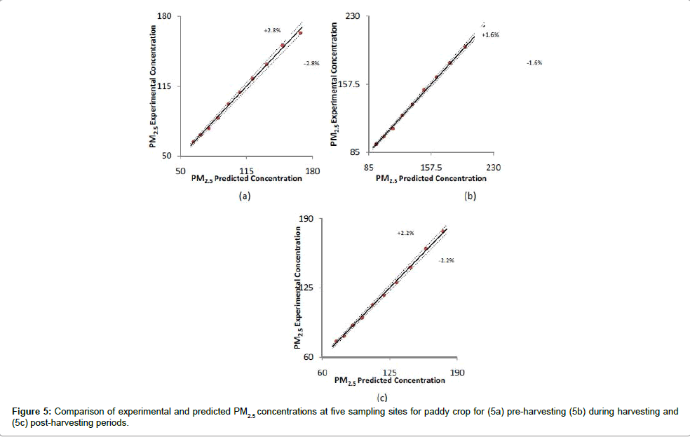
Figure 5: Comparison of experimental and predicted PM2.5 concentrations at five sampling sites for paddy crop for (5a) pre-harvesting (5b) during harvesting and (5c) post-harvesting periods.
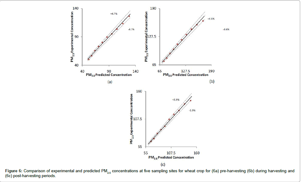
Figure 6: Comparison of experimental and predicted PM2.5 concentrations at five sampling sites for wheat crop for (6a) pre-harvesting (6b) during harvesting ansd (6c) post-harvesting periods.
The statistical parameters (R2, Mean, MPSD, RMSE, SSE and SE) using predicted values are determined by using their basic definitions and expressions available in literature [10] are presented in Tables 8 and 9 for paddy and wheat crops respectively.
| PM2.5 concentration for paddy crop | |||||||
| Sampling Periods | Statistical parameters | ||||||
| Regression Equation | R2 | Mean | MPSD | RMSE | SSE | SE | |
| Pre-Harvesting | y1=56.031e0.11x | 0.998 | 107.804 | 0.017 | 1.729 | 0.0001 | 1.921 |
| During harvesting | y1=85.246e0.0932x | 0.998 | 147.483 | 0.012 | 1.607 | 0.0007 | 1.769 |
| Post-Harvesting | y1= 66.763e0.0971x | 0.998 | 118.367 | 0.014 | 1.383 | 0.004 | 1.496 |
Table 8: Regression equation and statistical parameters for PM2.5 concentration for paddy crop.
| PM2.5 concentration for wheat crop | |||||||
| Sampling Periods | Statistical parameters | ||||||
| Regression Equation | R2 | Mean | MPSD | RMSE | SSE | SE | |
| Pre-Harvesting | y1=47.594e0.099x | 0.991 | 85.39 | 0.031 | 2.13 | 0.002 | 2.259 |
| During harvesting | y1=68.442e0.0909x | 0.992 | 116.721 | 0.024 | 3.084 | 0.0001 | 3.309 |
| Post-Harvesting | y1=60.451e0.0894x | 0.993 | 102.134 | 0.024 | 2.463 | 0.00001 | 2.684 |
Table 9: Regression equation and statistical parameters for PM2.5 concentration for wheat crop.
From these tables it is evident that RMSE values are quite low and hence, predictions of PM2.5 concentrations are in close agreement with the experimental PM2.5 concentrations.
From the analysis of both PM10 and PM2.5 concentrations, it is evident that crop residue burning does effects the PM10 and PM2.5 concentrations in ambient air during, pre- and post-harvesting periods and are observed in much higher concentrations (617.2 μg/m3 for PM10 and 176.3 μg/m3 for PM2.5), than the permissible standards of NAAQS (2009). As per NAAQS (2009), the PM10 concentration in ambient air is 100 μg/m3 (24hr Average) while PM2.5 concentration is 60 μg/m3 (24hr average) [8]. In order to predict the concentrations of PM10 and PM2.5 in ambient air for both paddy and wheat crops (pre-, during and postharvesting periods), non-linear regression equations (power function for PM10 and exponential function for PM2.5) are developed, which are found accurate in prediction of PM10 and PM2.5 concentrations in present work. However, they need to be verified with experimental results in future studies.
The primary objective of this study was to develop regression based models to predict the PM10 and PM2.5 concentrations in ambient air where crop residue burning is practiced. In the present work, using experimental results of PM10 and PM2.5, measured in Mandi- Gobindgarh (Punjab state) in India due to crop residue burning during, pre- and post-harvesting periods for paddy and wheat crops are utilized to develop non-linear regression models to predict PM10 and PM2.5 concentrations. PM10 concentrations are best described by a nonlinear power functions while PM2.5 concentrations are well described by exponential functions, as evident from high R2 values (R2>0.99) and low RMSE values in almost all cases studied. These regression equations are based on present experimental results, therefore, they need to be verified in future studies.
The authors are grateful to UPPCB, Lucknow and PPCB, Mandi-Gobindagrh for their support rendered in preparation of this manuscript. Authors would like to thank the Director, MNNIT, Allahabad and Head, School of Energy and Environment, Thapar University, Patiala for providing the required help for this paper.