Journal of Pollution Effects & Control
Open Access
ISSN: 2375-4397
ISSN: 2375-4397
Research Article - (2015) Volume 3, Issue 3
Nitrogen is an essential nutrient to form amino acids for fauna and flora. Its compound ammonia, however, is also one of the most important contaminants in an aquatic environment for its highly toxic nature and ubiquity in the surface water. Monitoring and controlling the total ammonia nitrogen are vital for human health and sustainable economic development. This paper attempts to develop an optimal model to monitor and predict the development of total ammonia nitrogen in a water body. A case study was carried out in the Houston Ship Channel and Galveston Bay in Texas, which aquatic environment is a nursery and spawning ground for diverse types of marine life. Meanwhile, the Bay also assimilates ammonia pollutants from Texas’s municipal and industrial wastewater. The toxic threat of total ammonia nitrogen in the bay was assessed, based on observed samples and forecasted values. Forty years of samples were collected from the Texas Commission on Environmental Quality. Correlations analysis was conducted between all physical, biological and chemical parameters and the total ammonia nitrogen. The trends of total ammonia nitrogen were modeled through a multivariate regression and an auto-regression, followed by an estimation of hazard quotient. The outcome shows that the total ammonia nitrogen in this study area is spatially correlated. For upstream flow, most measured parameters were highly correlated with the total ammonia nitrogen, whereas for downstream flow, weak correlations were noticed. Modeling results indicate that the auto-regression models can better fit the observed data than the multivariate regression models. Meanwhile, the predicted total ammonia nitrogen and the hazard quotient will remain at a lower level, meeting the ambient water criteria continuous concentration.
Keywords: Water pollution; Hazard quotient analysis; Time series model; Multivariate regression; Correlation analysis
TAN: Total Ammonia Nitrogen
Fauna and flora require nitrogen as an essential nutrient to form amino acids. These amino acids perform critical roles in processes, such as neurotransmitter transport and biosynthesis [1]. Even though 75% of the atmosphere is nitrogen in its diatomic form (N2 gas), few living creatures can utilize this type of nitrogen directly. Nitrogen needs to be converted into other forms before most aquatic plants can utilize it.
Ammonia (NH3), or azane, is one of the important sources of nitrogen for the living system. It contributes significantly to the nutritional needs of terrestrial organisms, serving as a precursor to food and fertilizers. Ammonia is widely used in many commercial cleaning products and is considered as one of the most important contaminants in an aquatic environment for its highly toxic nature and ubiquity [2]. Fish and amphibians lack a mechanism to prevent ammonia’s buildup in the bloodstream, like humans and other mammals do. They usually eliminate ammonia from their bodies by direct excretion. Therefore, ammonia is toxic to the aquatic environment, even at low concentrations.
NH3 is an unionized ammonia that can react with water to form ionized ammonia (NH4+) in a weak base; it is represented by the chemical equilibrium in Equation 1.
 (1)
(1)
The unionized ammonia and ionized ammonia exist simultaneously in the water; it can be measured as the total ammonia nitrogen (TAN). The proportion of NH3 in TAN is subject to the values of pH, temperature, and salinity in the aquatic environment [3-7]. The toxicity of TAN increases as the pH decreases, and as temperature decreases. The higher base leads to higher ionized ammonia, thereby increasing toxicity [8].
The toxic concentrations of NH3 range from 0.53 to 22.8 mg/L for freshwater organisms [8]. Though plants are more tolerant of ammonia than animals, the hatching and growth rates of fish may result in changes in the tissue of gill, liver, and kidney. For human beings, an excessive concentration of ammonia may cause a loss of equilibrium, convulsions, coma, and death. Therefore, to prevent any chronic and acute aquifer toxicity, a sufficient monitoring approach is required. A monitoring approach is usually referred to biological measurements at regular sites or random sites throughout an area and state, which are time-consuming work and cannot predict seasonal change in water quality. Modeling could complement these imperfections in the approach of biological measurements.
This paper attempts to develop an optimal model to monitor the dynamic TAN concentration in a water body and assess the toxic threat of TAN to the aquatic environment, based on a case study in the Houston ship channel and Galveston Bay (HSC&GB) in Texas (USA) was selected. The Bay assimilates ammonia pollutants from Texas’s wastewater discharge for more than 4.5 million populations; this includes raw or partially treated industrial wastes, and non-point source storm water runoff [9]. The overload of nutrients, fecal coliform bacteria, and suspended solids are attributed to deleterious effects on the HSC&GB’s water quality and aquatic life.
Since the late 1960’s and earlier 1970’s, many remediation plans have been implemented in the HSC&GB, such as wastewater treatment at the point sources and a federal/state permitting process [10]. Though the concentration of pollutants has been controlled, the monitoring of the nutrient dynamics is still required for sustainable economic development.
Sample collection
The data samples used in this paper were collected in the HSC&GB, in the State of Texas (USA). The Upper & Lower Galveston Bay is a shallow bay with an average depth of 7 feet (2.1 meters), a length of 35 miles (56 km), and a width of up to 19 miles (31 km). It is the largest estuary in Texas and the 7th largest estuary in the US. The Houston ship channel provides deep-water access to both the Gulf of Mexico and Houston [11]. The unique and complex mixing of water in this area provides important nursery and spawning grounds for diverse types of marine life, including crabs, shrimp, oysters, and fish. Consequently, this spawning ground contributes to Texas’ economy by 4.2 billion dollars annually [9].
The TAN observed concentrations for this research were obtained from the water database of the Texas Commission on Environmental Quality [12] from the early 1970’s until 2010. A total of 206 samples were collected from the Houston Ship Channel; 1978 samples were collected from the Upper & Lower Galveston Bay. The entire study area is divided into six groups, as illustrated in Figure 1.
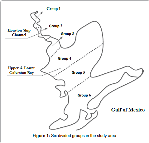
Figure 1: Six divided groups in the study area.
Analytical methods
Analytical procedure:The method to analyze and model the TAN in the HSC&GB is to follow a five-step procedure:
dividing the entire study area into six groups, as shown in Figure 1, and calculating the mean concentration for each group;
conducting time/spatial correlation analyses among the observation groups and a dependency correlation analyses to identify potential dependent parameters for modeling;
conducting multivariate regression modeling between the identified dependent variables and the TAN from relevant groups;
conducting time series modeling for the TAN from all groups; and
evaluating the toxic threat of ammonia to the aquatic environment by calculating the Hazard Quotient (HQ) of the TAN.
Correlation analyses: Due to the connected water body in the study area, the TAN concentration may be spatially correlated to each other. The spatial correlation analyses of TAN concentrations among observation groups will be conducted.
Besides, the un-ionized ammonia concentration is very sensitive to pH and temperature, which vary from time to time and season to season. The un-ionized ammonia concentration is often estimated through TAN. The dependency correlations between the TAN and the parameters indicating water and ecological quality were studied as well, including pH, temperature, Total Suspended Solids (TSS), Total Organic (TO), Chlorophyll a, salinity, Dissolved Oxygen (DO), orthophosphorus (OP), Biochemical Oxygen Demand (BOD), Specific Conductance (SC), fecal, and E coli, Enterococci. The cross analysis of dependency correlation attempts to identify potential dependent parameters for the TAN from each group.
Multivariate regression modeling: The multivariate regression attempts to determine a formula that can describe how elements in a vector of parameter (e.g., TAN) respond simultaneously to the changes in others (e.g., the parameters that may have higher correlation with TAN in the same group). The multivariate regression is distinct from the multivariable regression, which has only one dependent variable [13]. A multivariate normal regression is the regression of a multidimensional response on a design matrix of predictor variables, with normally distributed errors.
 (2)
(2)
where: yi (t) is the TAN for group i in year t, xij (t) is the jth parameters for the TAN of group i in year t. ni is the total number of parameters for group i. {αij} is the regression coefficients and ei is the error term following a normal distribution.
Time series modeling: No matter whether the dependent parameters can be successfully identified in step 1, the TAN from all groups can be treated as chronic datasets called “time series” with “no consideration of” the dependent parameters. The “raw” datasets should be pre-processed by removing the trend components from the TAN observations, while the residuals with a zero mean should be used for non-dependent parameter modeling [14].
The candidate “best fit” models include Autoregressive (AR) models and Moving Average (MA) models, or their combination ARMA model [14]. As the Moving Average (MA) part needs error information from real observations, which is not feasible during the forecasting stage, only the Autoregressive part as AR models are considered in this research.
Assuming xt is the TAN observation for year t, the estimate of xt can be expressed in Equation 2.
 (3)
(3)
In Equation (3), xt-i means the TAN observation in the ith year before year t.  are the coefficients of {xt}, i=1, 2, …n, n is the order of the model. can be calibrated using algorithms such as the Forward-Backward algorithm (FB), the Least Squares algorithm (LS), the Yule-Walker algorithm (YW), the Burg’s algorithm (BURG), and the geometric lattice method (GL) [14]. The goodness of the models is based on indexes such as the Akaike Information Criterion (AIC) (please refer to Akaike (1974) [15] for more AIC detail). The modeling error a follows an independent normal distribution
  .
.
Risk assessment: The toxic threat of ammonia to the aquatic environment in HSC&GB will be assessed by the Hazard Quotient (HQ) of TAN for each group, which is expressed as the concentration ratio between the observed and reference values (Equation (4)).
 (4)
(4)
The ambient water Criteria Continuous Concentration (CCC) for saltwater was adopted as the reference concentration. The CCC’s should be selected based on the water salinity level, pH values, and temperature in the different groups.
Characteristics of the TAN in the HSC&GB
The time spatial distribution of TAN concentrations in the HSC&GB is shown in Figure 2. The primary TAN pollutants sources come from the Houston Ship Channel, as the TAN concentrations in groups 1 and 2 (in the Ship Channel and up to 5 mg/l in mid-1970) are significantly are higher than others. The TAN concentrations in groups 4 and 5 (within the Galveston Bay) decrease to much less than 0.5 mg/l, which may be the result of the dilution of the seawater from the Gulf of Mexico. The TAN values in group 3 are in the middle.
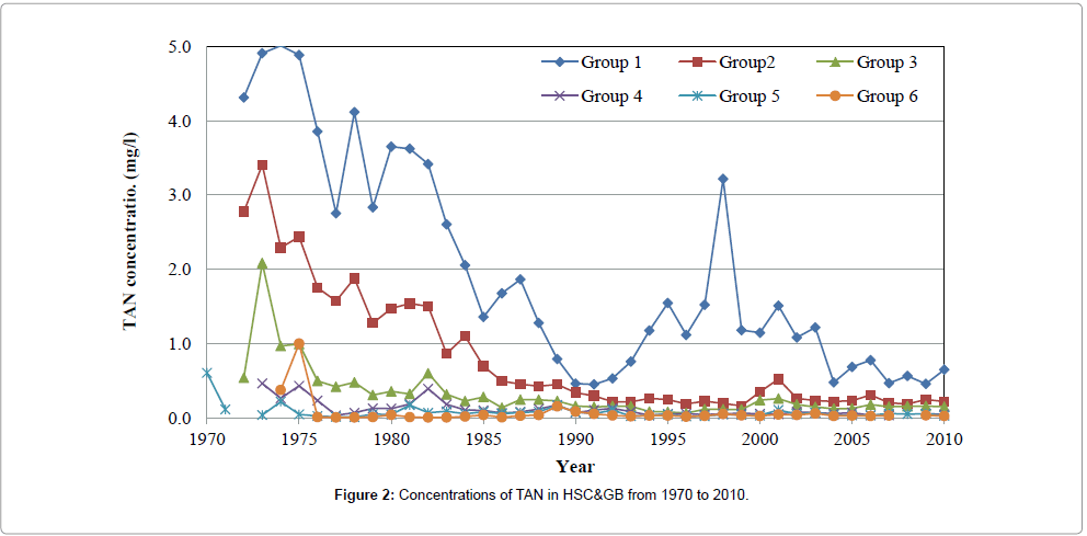
Figure 2: Concentrations of TAN in HSC&GB from 1970 to 2010.
Spatial correlation
The correlations of the TAN concentration among all six groups are listed in Table 1. Strong correlations are found between groups 1 & 2, 2 & 3, and 3 & 4 with correlation coefficients of 0.91, 0.86, and 0.80, respectively. The correlations between the first four groups (1-4) and the last two groups (5 and 6) are apparently weaker. The weakest correlation is between group 5 and the other five groups, ranging from 0.10 to 0.30.
| Group/Parameter | Group 1 | Group 2 | Group 3 | Group 4 | Group 5 | Group 6 | |
| Spatial Correlation | 1 | 0.91 | 0.73 | 0.63 | 0.10 | 0.36 | |
| 2 | 0.86 | 0.66 | 0.06 | 0.33 | |||
| 3 | 0.80 | 0.10 | 0.34 | ||||
| 4 | 0.30 | 0.51 | |||||
| 5 | 0.22 | ||||||
| Dependency Correlation | HSC1_pH | -0.04 | 0.02 | 0.37 | 0.30 | 0.01 | 0.24 |
| Total Suspended Solids (TSS) | 0.71 | 0.53 | 0.50 | 0.15 | -0.06 | 0.08 | |
| Total Organic (TO) | 0.71 | 0.06 | -0.11 | 0.32 | 0.06 | 0.21 | |
| Chlorophyll a | 0.21 | 0.59 | 0.69 | 0.54 | -0.06 | -0.46 | |
| Salinity | -0.20 | 0.21 | 0.27 | -0.04 | -0.05 | -0.15 | |
| Temperature | -0.13 | MD | 0.05 | -0.03 | 0.07 | -0.03 | |
| Dissolved Oxy (DO) | -0.80 | -0.71 | -0.14 | 0.09 | -0.19 | 0.22 | |
| Ortho-Phosphorus (OP) | 0.61 | 0.91 | 0.75 | 0.59 | -0.26 | 0.65 | |
| Biochemical Oxygen Demand (BOD) | 0.65* | 0.11 | 0.67* | 0.26 | 0.03 | 0.40 | |
| Specific Conductance (SC) | 0.02 | -0.09 | -0.28 | -0.19 | -0.15 | -0.34 | |
| Fecal | MD | MD | MD | -0.02 | 0.36 | 0.01 | |
| E coli | MD | MD | MD | MD | MD | MD | |
| Enterococci | MD | MD | MD | 0.51* | -0.14 | -0.09 | |
| Total Nitrate Nitrite Nitrogen (TN) | -0.61 | -0.26 | 0.69 | 0.09 | 0.35 | -0.10 |
Table 1: Spatial correlation and the correlation between the TAN concentrations and the other physical, biological and chemical parameters.
Dependency correlation
Ammonia in an aquatic environment is sensitive to many factors. Therefore, it is necessary to conduct a correlation analyses between the TAN and related physical, biological and chemical parameters. Their correlation results are listed in Table 1.
In Table 1, apparently almost all correlation coefficients for groups 4 to 6 (all in Galveston Bay area) are less than 0.5, which implies that, in the Galveston Bay area, the TAN is not well correlated with all of the listed parameters. It is more likely that Galveston Bay pays a crucial role in the dilution and degradation of contaminants coming from the Houston Ship Channel.
By excluding the parameters with continuously missing data, the dependent variables for TAN are: TSS, TO, DO, Ortho-Phosphorus, and TN for group 1; TSS, Chlorophylla, DO, and Ortho-Phosphorus for group 2; TSS, Chlorophylla, Ortho-Phosphorus, and TN for group 3; and Chlorophylla and Ortho-Phosphorus for group 4.
From the modeling perspective for groups 1 to 4, multivariate regression models could be an option to depict the relationships between TAN and its correlated parameters. For groups 5 to 6, since there is no significant independent variable identified, the time series model, especially the auto-regression (AR) model, could be a possible choice. The AR models could also be applied to TANs for groups 1 to 3, as long as the modeling errors are acceptable.
Multivariate regression modeling for groups 1 to 4
Figures 3a-3d show the observed and MR predicted TANs for Groups 1 to 4, respectively. At first glance, the MR modeled values can basically catch the trends of the observed TANs. The calibrated coefficients of all MR models are listed in Table 2.
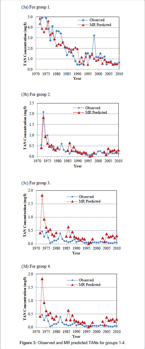
Figure 3: Observed and MR predicted TANs for groups 1-4.
| Parameters | Group 1 | Group 2 | Group 3 | Group 4 |
| Total Suspended Solids (TSS) | 0.035976672 | 0.016241028 | -0.005974875 | N/A |
| Total Organic (TO) | 0.065535998 | N/A | N/A | N/A |
| Chlorophylla | N/A | 0.006295538 | 0.009072259 | 0.000118654 |
| Dissolved Oxy (DO) | -0.161808029 | -0.098797239 | N/A | N/A |
| Ortho-Phosphorus (OP) | 0.528104801 | 0.95821269 | 0.4602417 | 0.00872595 |
| Total Nitrate Nitrite Nitrogen (TN) | 0.080082469 | N/A | 0.243803128 | N/A |
Table 2: Calibrated coefficients α_ of all MR models.
Time series modeling for all groups
The chronic TAN for each group from 1970 to 2010 is a time series. Even though the MR models have been applied to the modeling of the TANs for groups 1 to 3, time series could be an ideal alternative to model them and compare the modeling errors. Therefore, the time series modeling process is applied to the TANs for all groups (i.e., groups 1 to 6).
In this sense, the time series models will be built up with no dependent variables during the modeling process, which follows a four-step procedure: (1) spatial correlation analyses among observation groups; (2) dependency correlation analyses for potential dependent variables; (3) removal of trend components from the TAN observations; and (4) the time series modeling for the residuals of the TAN observations with the trend components removed.
The first two steps are to understand the correlations of the TAN spatially and with other possible dependent factors; while the last two steps are the standard processes of time series modeling [16].
Removing the determinative trends from the TAN sets: One pre-requisite of time series modeling is to remove the known determinative trends, as well as the mean values, from the datasets. The typical determinative trends to consider include exponential functions, linear functions, and Sine functions. The de-trended residuals should go through a de-mean process to make sure the residual datasets are with the zero mean. The identified determinative trends for all groups are listed in Table 3.
| Group | Component | Equations |
| 1 | Exponential |  |
| Linear |  |
|
| De-mean |  |
|
| Time Series | 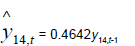 |
|
| 2 | Exponential | 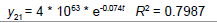 |
| Linear |  |
|
| De-mean | 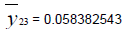 |
|
| Time Series | 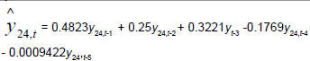 |
|
| 3 | Exponential | 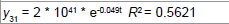 |
| Linear |  |
|
| De-mean |  |
|
| Time Series | 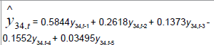 |
|
| 4 | Linear |  |
| De-mean |  |
|
| Time Series | 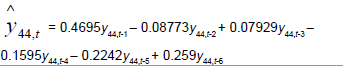 |
|
| 5 | Exponential | 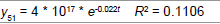 |
| Linear |  |
|
| De-mean | 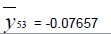 |
|
| Time Series | 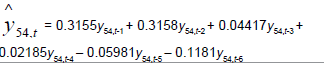 |
|
| 6 | Exponential |  |
| Linear |  |
|
| De-mean |  |
|
| Time Series |  |
Table 3: Identified determinative trends and time series models for groups 1-6.
Time series modeling results: The de-trended and time series modeling equations are listed in Table 3. The observed and AR predicted TAN for groups 1 to 6 are illustrated in Figures 4a-4f, respectively, which shows that the predicted values were very close to the observed one. Their modeling errors are discussed in the following section.
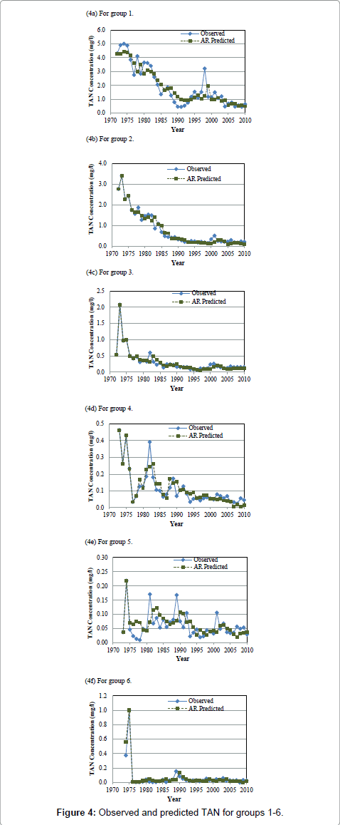
Figure 4: Observed and predicted TAN for groups 1-6.
Discussion of the modeling: The orders of time series modeling, AIC values, and the Root Mean Squared Deviation (RMSD) of AR modeling errors for all six groups, plus the RMSD for all MR models, are listed in Table 4.
| Group | MR Models | AR Models | ||
| RMSD | Order | AIC | RMSD | |
| 1 | 0.794 | AR(1) | -1.013 | 0.581 |
| 2 | 0.528 | AR(5) | -3.344 | 0.153 |
| 3 | 0.198 | AR(5) | -4.748 | 0.076 |
| 4 | 0.284 | AR(6) | -5.931 | 0.039 |
| 5 | AR(6) | -6.241 | 0.036 | |
| 6 | AR(3) | -6.961 | 0.040 | |
Table 4: Comparison of the modeling RMSDs.
For groups 1 to 4 in Table 4, the RMSDs of AR are all smaller than their corresponding ones for MR. This means that the time series modeling errors are all less than the multivariate regression ones. Therefore, time series models (the AR models) are adopted for modeling the TANs of all groups. The equations in Table 3 can be used to model the TANs from 1970 until 2010, and even forecast the future year’s TAN.
Characteristics of the water body in HSC& GB
Over forty years, there is trend of decline in TAN, TSS, chlorophyll a, ortho-P, and TO, while DO increased. These are the sign of better water quality.
Table 5 lists the mean values and standard deviations of all observed parameters. From Group 1 to 6, the pH and temperature were stable, whereas the salinity, SC, and TSS increased visibly. The closer to the Gulf of Mexico, the water becomes saltier, more dissolved solids (such as salt), and more organic and inorganic particles dispersed in water. The increased DO indicates less contaminant that induces oxygen consumption in the group closely the Gulf. On the contrary, the TO, TAN, Orthor-P, BOD, TN declined obviously, which indicate the decrease in total organic and inorganic matters, nutrients, and biological organisms in the water body closer to the Gulf. Besides, Chlorophll a in group 3-5 were apparently higher than those in other groups, which indicates higher phytoplankton abundance and biomass as well as poor water quality.
| Parameter | Group 1 | Group 2 | Group 3 | Group 4 | Group 5 | Group 6 | ||||||
| mean | std | mean | std | mean | std | mean | std | mean | std | mean | std | |
| pH | 7,33 | 0,18 | 7,55 | 0,17 | 7,96 | 0,21 | 8,17 | 0,19 | 8,18 | 0,17 | 8,12 | 0,22 |
| TSS | 26,45 | 16,65 | 23,20 | 8,13 | 28,52 | 10,67 | 26,96 | 10,11 | 33,50 | 24,11 | 34,38 | 21,60 |
| TO | 11,36 | 5,84 | 16,08 | 2,83 | 16,69 | 3,13 | 6,62 | 4,41 | 5,30 | 4,13 | 5,04 | 3,99 |
| Chlorophylla | 6,03 | 3,65 | 8,75 | 7,33 | 13,72 | 10,94 | 18,18 | 18,70 | 12,21 | 14,51 | 6,80 | 5,45 |
| Salinity | 3,76 | 1,65 | 8,69 | 2,90 | 11,61 | 3,21 | 12,86 | 4,07 | 15,78 | 3,87 | 16,73 | 4,75 |
| Temperature | 23,58 | 1,61 | 23,00 | 1,59 | 22,80 | 1,78 | 22,24 | 1,75 | 22,39 | 1,58 | 22,40 | 2,24 |
| DO | 3,76 | 1,56 | 5,13 | 1,61 | 7,38 | 1,32 | 8,48 | 0,76 | 8,35 | 0,69 | 8,24 | 0,57 |
| Ortho-P | 1,32 | 0,63 | 0,95 | 0,62 | 0,53 | 0,31 | 0,39 | 0,23 | 0,18 | 0,28 | 0,20 | 0,24 |
| BOD | 5,96 | 2,92 | 3,83 | 1,52 | 4,26 | 1,55 | 4,17 | 1,71 | 3,88 | 1,95 | 4,31 | 2,26 |
| SC | 6909,11 | 2393,74 | 13911,72 | 4344,22 | 18089,14 | 4691,22 | 20815,20 | 5318,22 | 24535,18 | 5784,32 | 25846,60 | 6766,73 |
| TAN | 1,95 | 1,45 | 0,81 | 0,84 | 0,32 | 0,36 | 0,12 | 0,11 | 0,08 | 0,10 | 0,07 | 0,17 |
| Total Nitrogen | 1,40 | 1,01 | 1,29 | 2,37 | 0,59 | 0,87 | 0,18 | 0,08 | 0,11 | 0,07 | 0,06 | 0,07 |
Table 5: Mean values of all parameters over forty years in HSC& GB.
Further, the larger standard deviation of TSS, TO, and SC depict that the organic and inorganic particles, total organic, and dissolved solids in the water varied from year to year greatly.
Risk assessment of the TAN for the aquatic environment in HSC&GB
The total ammonia nitrogen Criteria Continuous Concentration (CCC) for each group was identified, according to the water salinity level, pH values, and temperature. In the last four decades, the salinity concentrations ranged between 4 g/kg and 12 g/kg in Group 1 to 3, and 13 g/kg and 17 g/kg in Group 4 to 6, respectively. Saltwater with a salinity of 10 g/kg and 20 g/kg was adopted in the estimation of the Hazard Quotient (HQ) for group 1-3, and group 4-6, respectively. The overview of the HQ is illustrated in Figure 5.
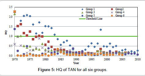
Figure 5: HQ of TAN for all six groups.
In Figure 5, the samples displayed above the threshold line indicate that the opportunity of toxic effects caused by ammonia to the aquatic environment is relatively high, while below the line represents a lower possibility. In the 1970’s, there was higher risk taking place in groups 1 and 2 (Houston Ship Channel). This implies that the TAN seriously contaminated the water body. In fact, in that period, the water quality had raised a great concern, which motivates the implementation of various plans to monitor and remedy the freshwater in HSC&GB.
In the 1990’s, the HQ increased dramatically, crossing the 6 groups. In the last two decades, the HQ in group 1 fluctuated slightly, but was still below the threshold line.
This substantial decline may be attributed to the great success of the remediation plans. Moreover, the plans also contribute to the maintenance and monitoring of the water quality in the last two decades. The HQ in the rest of the groups remained stable, as less than 0.25. In other words, since the 1990’s, the water quality in the HSC&GB has improved significantly, and therefore, the toxic threat of the TAN to the aquatic environment was lessened.
The identified models were further used to predict the TAN concentrations for the year of 2011, which is still not available in the public. The predicted TAN in 2011, together with the compared 2010 observations and the related HQ, are listed in Table 6.
| Parameters | Group 1 | Group 2 | Group 3 | Group 4 | Group 5 | Group 6 |
| Salinity concentrations (g/kg) | 4-12 | 13-17 | ||||
| Saltwater salinity criteria (g/kg) | 10 | 20 | ||||
| T oC (2010) | 20 | 20 | 20 | 20 | 20 | 20 |
| pH (2010) | 7.6 | 7.8 | 8 | 8.4 | 8.4 | 8.4 |
| CCC* (mg/l) | 2.4 | 1.5 | 0.97 | 0.44 | 0.44 | 0.44 |
| TAN (mg/l)(2010) | 0.65 | 0.22 | 0.15 | 0.05 | 0.03 | 0.03 |
| HQ (2010) | 2.71E-01 | 1.47E-01 | 1.55E-01 | 1.14E-01 | 6.82E-02 | 6.82E-02 |
| TAN (mg/l)(2011) | 0.52 | 0.06 | 0.07 | 0.00 | 0.02 | 0.01 |
| HQ (2011) | 2.17E-01 | 4.00E-02 | 7.22E-02 | 2.27E-04 | 4.55E-02 | 2.27E-02 |
Table 6: Identification of toxicity criteria for each group and HQ estimation for2010 and 2011.
Table 6 shows that the TAN observations in the both the years of 2010 (observed) and 2011 (forecasted) for all groups were lower than the corresponding CCC. Their Hazard Quotient (HQ) values were also relatively lower, between 2.27E-04 and 2.71E-01. This means that the toxic threat of ammonia to the aquatic environment is low. The remediation plans for wastewater treatment proposed in the late 1960’s and early 1970’s continue to contribute to the water quality in the Houston ship channel and Galveston Bay in Texas (USA).
In this investigation, the TAN concentration in the divided six groups of the HSC&GB were analyzed and modeled. Since the implementation of remediation plans in the late 1960’s and earlier 1970’s, the water quality has significantly improved. The treatment at the point sources has made a great contribution. The correlation results show that the TAN concentration is highly correlated to the different geo-locations. This phenomenon could be the result of the higher capacity of dilution and degradation that the upper and lower Galveston Bay possesses. For the upstream flow, there were 2-4 parameters that were highly correlated with TAN (R>0.50), while for the downstream flow, weak correlations were noticed between the TAN and the 14 candidate parameters. By eliminating the parameters with the continuously missing data, the highly correlated parameters were chosen as dependent variables to model the chronic TAN concentrations using a multivariate regression (MR) in groups 1 to 4. On the other hand, the time series AR models were applied to all groups. The results show that the AR is able to model and predict the trends of the TAN more accurately than the MR. The predicted TAN and the HQ will remain at a lower level, meeting the ambient water Criteria Continuous Concentration (CCC).
The author sincerely appreciates the detailed instructions from Dr. Maruthi Sridhar B. Bhaskar on data processing. The author also wishes to acknowledge the supports in part by the US. Tier 1 University Transportation Center TranLIVE # DTRT12GUTC17/KLK900-SB-003, and the U.S. National Science Foundation (NSF) under grant #1137732.