Journal of Aeronautics & Aerospace Engineering
Open Access

Minimum-Fuel, Low-Thrust Trajectory Optimizations for Earth-to-Mars Orbit Transfer with Bang-Bang Control

Daero Lee^{* *}Correspondence: Daero Lee, Department of Aerospace Science Engineering, Tuskegee University, Tuskegee, USA, Email:

Author info »

Introduction

Electric propulsion systems have demonstrated that low-thrust engines have the capability to be used for long-duration travels by the planetary and interplanetary space missions. Electric propulsion has been used by NASA’s deep space 1 and Dawn, ESA’s SMART-1 and JAXA’s Hayabusa and Hayabusa 2 [1-4]. Low-thrust electric propulsion spacecraft is known to have a greater payload capability than conventional chemical propulsion spacecraft. Low-thrust propulsion is very effective for long-duration of interplanetary space missions but the corresponding problem is computationally challenging to solve [5]. Low-thrust trajectory optimization generally accompanies determining the control variables, which may include thrust magnitude and direction and parameter and the corresponding trajectories while minimizing a given performance index (propellant consumption or time-of-flight) and satisfying boundary conditions (departure and arrival orbits), mid-point conditions and path constraints.

The optimizations of low-thrust trajectories have been mathematically formulated as an optimal trajectory design (OCP) [6]. In general, the techniques to any optimization problems can be divided into two categories: Direct method and indirect method [7]. Indirect method solves the optimal trajectory design by obtaining the solution to the corresponding Two-Point Boundary-Value Problem (TPBVP) which results from the calculus of variations. The application of the Lagrange multipliers (costates) doubles the number of differential equations that have to be integrated along the trajectory. However, the solution to the TPBVP is very sensitive to initial guess for costate variables which do have any intuitive physical meanings. In contrast, direct method solves the optimal trajectory design by converting it into a Nonlinear Programming (NLP) problem with various transaction schemes applied to either states and controls or both states and controls. Since the control variables are explicitly parameterized, a good initial control guess for direct methods can be easily produced. In addition, the modifications of the performance index, equality constraints, state and control inequality constraints can be easily made for different problem formulations in direct method while a new derivation of TPBVP should be obtained in indirect method.

Many studies have been progressed for fuel-optimal low-thrust interplanetary trajectory optimization by both indirect methods and direct methods. In indirect methods, Valadi and Nah treated fuel-optimal trajectories for rockets powered by lowthrust propulsion with variable specific impulse [8]. The optimal trajectory design is solved using an indirect, multiple shooting method. Jiang et al. presented the fuel-optimal problem of lowthrust trajectory by the homotopic approach combined with the single shooting method as an indirect method [9]. Two examples of fuel-optimal rendezvous problems from the Earth directly to Venus and from the Earth to Jupiter via Mars gravity assist with the constant specific impulse for Bang-Bang control were given to substantiate the perfect efficiency of these techniques [10,11]. Chi et al., presented a series of optimization methods as indirect methods for finding fuel-optimal gravity-assist trajectories that use the practical solar electric propulsion with variable specific impulse [12]. The fuel-optimal low-thrust gravity-assist trajectories are first solved using specific impulse as a control variable. Zhu et al. demonstrated a novel continuation technique to solve optimal bang-bang control for low-thrust orbital transfers that take into account the first order necessary optimality conditions [13]. In direct methods, Tang and Conway and applied the method of collocation with nonlinear programming to the determination of minimum-time, low-thrust interplanetary transfer trajectories [14,15]. Patterson and Rao solved the orbit-raising optimal trajectory design taken from Bryson and Ho with GPOPS-II [16,17]. Guo et al. showed the application of hp-adaptive pseudospectral method in the solar sail minimum time Earth-Mars transfer trajectory optimization [18].

In this paper, the governing equations of the motion are normalized for the fundamental distance, velocity, mass and time to streamline the numerical computations. In the indirect method, the analytical formulations of the problem are presented to set up TPBVP using the primer vector theory and the necessary conditions for an optimal solution are discussed. In the direct method, the bounds of the states, the flight time and the control including the maximum available power, the equality constraint and the boundary conditions are explicitly specified. The optimal control problem is converted to the parameter optimization problem that can be solved by Nonlinear Programming (NLP). General-purpose optimal control software called GPOPS-II is adopted to solve optimal trajectory design using variable-order Gaussian quadrature collocation methods where the continuous-time optimal trajectory design is transcribed to a large sparse nonlinear programming problem [19]. Then, the solutions of this problem at the different flight time and maximum input powers of the spacecraft will be compared and validated for different mission scenarios. Numerical studies show that the fuel-optimal, lowthrust heliocentric Earth-to-Mars trajectories for the specific arrival time and maximum power are obtained with different thrust magnitudes with “on-off-on” thrusting sequence. The primer vector theory is employed to analyze the Bang-Bang control structure by monitoring the variations of the switching functions.

This paper develops minimum-fuel, two-dimensional low-thrust trajectory optimization methods for the spacecraft with a constant specific impulse engine to apply for Earth-to-Mars orbit transfer using direct method and indirect method. The trajectory optimization problems are solved in the heliocentric frame with bang-bang control structure to obtain minimum-fuel, two-dimensional low-thrust Earth-to-Mars trajectories. The optimal solutions of the two optimization methods are validated with the primer vector theory and their numerical matching. Finally, the solutions are also validated for different flight time and maximum input powers.

Materials and Methods

Problem formulation

In this section, the governing equations of motion are given in the two-dimensional polar coordinate and the normalized equations of motion are also given. The spacecraft is propelled by electric propulsion with a constant CSI engine.

Equations of motion: This trajectory optimization problem is modeled in a two-dimensional, heliocentric (sun-centered) polar coordinate system to make the optimization methods more efficient and robust instead of Cartesian coordinates which is the simplest but most disadvantageous choice [20]. All motions are assumed to be confined to the ecliptic or fundamental plane. Figure 1 illustrates the geometry of this coordinate system along with the steering angle.

Figure 1: Geometry of heliocentric coordinate system along with the steering angle.

Where r is the heliocentric radius of the spacecraft, θ is the phase angle, υ_r and υ_θ are the radial and transverse velocity components, respectively and α is the steering or thrust orientation angle. The steering angle is measured relative to the instantaneous tangential direction and is positive in the clockwise direction to the thrust vector. The two-dimensional equations of motion for the spacecraft in the polar coordinate system [21,22].

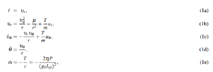
where m is time varying spacecraft mass, ur and uθ are the unit vector components in the thrust vector, μ is the solar gravitational constant, which equals to 1.32712441933 × 10¹¹ km³/s², T is the thrust of the low-thrust system and g₀=9.80665 m/s² is the standard gravitational acceleration. Most variables in equation m^. are engine specifications: η is the engine efficiency, P is the power and I_sp is the specific impulse. The power P is considered to be a variable which ranges from 0 to P_max, that is 0 ≤ P ≤ P_max. The thrust magnitude is defined as:

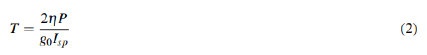
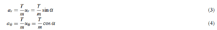
The above equation shows that the thrust magnitude and specific impulse are inversely proportional. In this study, the engine efficiency is assumed to be constant while the thrust is generated. The radial and tangential acceleration components due to thrust are defined as:

The boundary conditions and the inequality should be specified for a complete optimization problem. Here, the initial boundary conditions can be formulated as:

while the terminal boundary conditions are given by:

where tf is the predefined final flight time. The first equation in Eq. (6) states that the radial velocity should be zero and the second equation is a boundary condition is that forces the final velocity to be equal to the local circular velocity at the final radial distance. The equality path constraint is given by:

Normalized equations of motion: In summary, the normalized equations of the motion are given by:

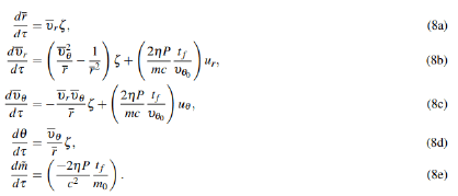
where the derivations for the normalized equation of motion are given in appendix. The normalized initial boundary conditions can be formulated as:

While the normalized terminal boundary conditions are given by:

Fuel-optimal optimal control

The fuel-optimal optimal control using a CSI engine is solved by the indirect method and the direct method, respectively. The thrust level is determined by the engine power P (0 ≤ P ≤ P_max). The input power is always limited by the availability of the power and the exhaust velocity is constant. From the given initial time t0 and the final rendezvous time t_f, the fuel-optimal trajectory design problem is to determine the history of thrust direction u(t) and the input power P that minimizes the scalar performance index or cost function given by:

subject to the powered equation of motion (8) while satisfying the boundary conditions of (9) and (10).

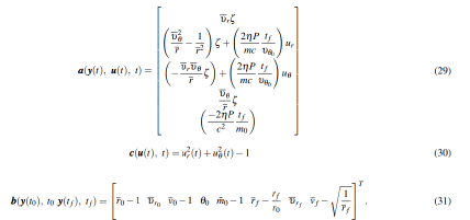
Indirect method: For an indirect method solution, a welldefined TPBVP for the normalized equation of motion (8) and the boundary conditions (9) and (10) is posed. As the first step, the Pontryagin’s Minimum Principle (PMP) [12], [22] is applied to formulate the Hamiltonian given by:

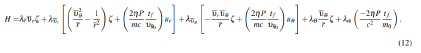
Where,

are the costate variables adjoint to the normalized radius, radial velocity, θ, normalized transverse velocity and mass, respectively.

Where,

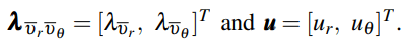
According to PMP, the optimal control is derived to minimize the Hamiltonian over the choice of the thrust direction by aligning the unit vector u(t) opposite to the adjoint vector,

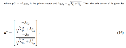
and the primer vector p(t) is defined, so that

for which,

The two terms in the square bracket of the Hamiltonian in Eq. (13) is written as H′

Equation (17) is usually rewritten as:

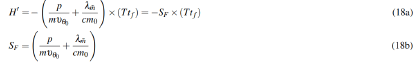
and the sign of the switching function SF determines when the thruster is turned on or off. The choice of the input power, P that minimizes the Hamiltonian in Eq. (17) is then given by the bang-bang control law:

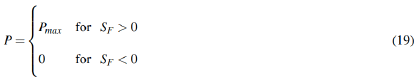
The maximum available power is adopted when S_F<0, whereas the engine is switched off when S_F<0 to minimize H′, according to the PMP. In addition, the thrust magnitude for 0 ≤ T ≤ T_max will also depend on the algebraic sign of the switching function S_F.

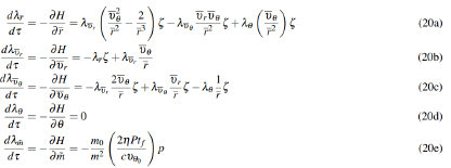
The Euler-Lagrange equations yield:

From the known initial conditions in Eq. (9) with the known initial time t₀=0 s and the known final conditions in Eq. (10) with the known final time t_f, ten boundary conditions can be obtained. The transversality condition is applied to pose a welldefined TBPVP.

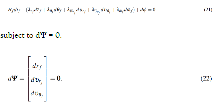
Expanding the nonzero terms in Eq. (22) while noting that we have a Mayer form of the performance index, where,

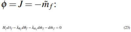
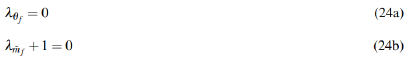
Using the the terminal boundary conditions, we get the following boundary conditions:

Substituting Eq. (16) into Eq. (8) and reiterating all differential equations and boundary conditions give the well-defined TPBVP:

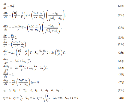
with τ ∈ [0,1]. The above formulation and the parameterization of the time and allows TPBVP solver known as bvp4c of MATLAB to solve the TPBVP (25) with the assumed initial and final dimensional times (τ₀) and (τ_f=1).

Direct collocation pseudospectral methods: In the direct collocation psedospectral method [16], the continuous-time optimal control problem is transcribed to a finite dimensional nonlinear programming problem using well-known software. To solve this minimum-fuel, low-thrust trajectory optimization problem with strict constraints, GPOPS-II which adopts a Legendre-Gauss-Radau quadrature orthogonal collocation method [19] is used. The continuous-time optimal control problem is transcribed to a large sparse NLP. The resulting NLP is then solved by well-known software, SNOPT [23]. Minimization of the cost function (11) is subject to the dynamic constraints (8) and the equality path constraint,

and boundary condition function are given as:

In this problem, the continuous-time state variables and control variable are given, respectively as:

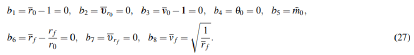
where the input power P is also included as a control variable which can be 0 or P_max. Unlike the indirect method, P appears explicitly in the problem formulation. The right-hand side function of the dynamics, the path constraint function, and the boundary functions are written, respectively, as:

Finally, the lower and upper bounds on the path constraints and boundary conditions are all zero. Because the first seven boundary conditions, (b₁,...b₈), are simple bounds on the initial and final continuous-time state, they will be enforced in the NLP as simple bounds on the NLP variables corresponding to the initial and terminal state. The 8^th boundary condition, b8, on the other hand, is a nonlinear function of the terminal state and thus, will be enforced in the NLP as a nonlinear constraint. The NLP occuring from the Radau pseudospectral discretization of the optimal control problem given in Eq. (11) and Eqs. (29)- (31) was solved NLP solver SNOPT.

Results and Discussion

Numerical results

In this section, the scenarios of the planar Earth-to-Mars orbit transfer for the spacecraft with the constant specific impulse engine were chosen to validate minimum-fuel, low-thrust trajectory optimization at three different input powers and the flight times. The Earth-to-Mars orbit transfer problem is applied for a rendezvous problem to reach the Mars orbit while the initial and final flight times are fixed. For this goal, the direct method and indirect method are used to solve the same problem and their solutions are compared. The initial and final orbital parameters are listed in Table 1. It is observed that the final position in the mission orbit (Mars orbit) is not specified since the purpose of these simulations is to reach the orbit not the Mars. As the forces acting on the spacecraft, the Sun’s gravity and the thrust produced by the engines are considered. The spacecraft is assumed to have initial mass 1500 kg and the CSI engine with Isp=3300 s and the constant thruster efficiency, η=0.7. The used input powers and the corresponding flight time are listed in Table 2. The input powers and flight time conditions of the scenario 1, 2 and 3 are listed in Table 2. The scenario 1 has 19 kW of input power and 240 days of flight time, the scenario 2 has 7.5 kW of input power and 365 days of flight time and the scenario 3 has 3.6 kW of input power and 2 years of flight time.

Table 1: Earth and Mars orbits for the evaluations of the optimization methods.

Table 2: Input powers (P) and flight times (tf)

Figure 2 shows the solution to the scenario 1 using GPOS-II with NLP solver SNOPT and a mesh refinement tolerance 10-8. The circle in this Figure 2 represents the locations of collocations by a variable-order adaptive pseudospectral method [24]. The dimensional state variables in Eq. (1) are plotted in Figure 2 (a). The unit vector of the thrust as the low-thrust transfer control variables, the in-plane thrust angle and the control acceleration are plotted in Figure 2 (b), (c) and (d). Between 88.9 days and 155 days, the control acceleration is zero, the spacecraft mass is constant and the control is discontinuous while the thrust is off. Figure 2 (e) shows an optimal low-thrust Earth-to-Mars transfer trajectory in the heliocentric coordinate with the Earth and Mars orbits. It shows the trajectory in black curve with the red arrows representing the thrust magnitude and direction. Figure 2 (f) shows a switching-function computed with Eq. (18b) for a two-burn sequence and thrust profile following the bang-bang control law by Lawden’s primer vector theory. In general, costate variables in an direct method is not computed in a direct method. However, GPOPS-II provides the costate variables which are used to compute the switching function (18b). Figure 2 (g) shows the thrust and input profiles where the maximum input power was constantly used by 19 kW while the switching function was positive. Figure 2 (h) show the mesh refinement history with ”hp-PattersonRao” method [19], [24]. Figure 3 shows the solution to the scenario 1 using bvp4c of MATLAB as the TPBVP solver in an indirect method when 10,000 mesh points are used. The dimensional state variables in Eq. (1) are plotted in Figure 3 (a). The unit vector of the thrust as the low-thrust transfer control variables, the in-plane thrust angle and the control acceleration are plotted in Figure 3 (b), (c) and (d), respectively. Between 88.9 days and 155 days, the control acceleration is zero and the spacecraft mass is constant while the in-plane thrust angle changes smoothly unlike the inplane thrust angle change in Figure 2 (c). However, it is due to numerical computation difference which is not remarkable. Figure 3 (e) shows an optimal low-thrust Earth-to-Mars transfer trajectory in the heliocentric coordinate with the Earth and Mars orbits, which matches with the one in Figure 2 (e) by GPOPS-II. The thrust direction in the trajectory represented with the red arrows is not clearly visible due to so many numbers of mesh points. But they show clear unit vector direction along the trajectory when they are magnified. Figure 3 (f) shows a switching-function for a two-burn sequence and thrust profile using Eq. (18b), which follows the Bang-Bang control law and matches with the result in Figure 2 (f). Thus, the solutions to the scenario 1 using the direct method and indirect method are numerically matching.

Figure 2: Solution to the scenario 1 using GPOS-II with NLP solver SNOPT and a mesh refinement tolerance 10-8.

Figure 3: Solution to the scenario 1 using bvp4c of MATLAB.

Figure 4 shows the solution to the scenario 3 using GPOS-II with NLP solver SNOPT and a mesh refinement tolerance 10−8. The dimensional state variables in Eq. (1) are plotted in Figure 4 (a) for 2 years longer than the flight time in Figure 2. The unit vector of the thrust as the low-thrust transfer control variables, the in-plane thrust angle and the control acceleration are plotted in Figure 2 (b), (c) and (d). Between 505.3 days and 653.2 days, the control acceleration is zero, the spacecraft mass is constant and the control is discontinuous while the thrust is off. Figure 4 (e) shows an optimal low-thrust Earth-to-Mars transfer trajectory in the heliocentric coordinate with the Earth and Mars orbits while more than one spiral trajectory around the Sun was generated. Figure 4 (f) shows a switching-function computed with Eq. (18b) for a two-burn sequence and thrust profile following the bang-bang control law. The thrust profile is thruston- off-on sequence depending on the sign of the switching function SF. Figure 4 (g) shows the thrust and input profiles where the maximum input power was constantly used by 3.6 kW while the switching function was positive. Figure 4 (h) show the mesh refinement history with more mesh point locations than those of Figure 2 (h).

Figure 4: Solution to the scenario 3 using GPOS-II with NLP solver SNOPT and a mesh refinement tolerance 10⁻⁸.

Figure 5 shows the solution to the scenario 3 using bvp4c of MATLAB as the TPBVP solver in an indirect method when 15,000 mesh points are used. The state variables in Figure 5 (a) match with the state variables in Figure 4 (a). The control unit vector u(t) and in-plane thrust angle are shown in Figure 4 (b) and (c). The control acceleration is zero and the spacecraft mass is constant between 505.3 days and 653.2 days. Figure 5 (e) shows an optimal low-thrust Earth-to-Mars transfer trajectory in the heliocentric coordinate with the Earth and Mars orbits, which matches with the trajectory in Figure 4 (e). The thrust direction in the trajectory represented with the red arrows are not clear either due to so many numbers of mesh points. But they show clear direction along the trajectory when they are magnified. Figure 5 (f) shows a switching-function for a two-burn sequence and thrust profile, which matches with the result in Figure 4 (f). It is obvious to observe the thrust is off while the switching function SF is negative and the thrust is on while the switching function SF is positive. Therefore, the solutions to the scenario 3 using the direct method and indirect method are also numerically matching like the solutions to the scenario 3 using the both methods.

Figure 5: Solution to the scenario 3 using bvp4c of MATLAB.

However, the solutions to scenario 2 are not given by the figure results. Instead, the solution values using both the direct and indirect methods are listed in Table 3. It shows the Δ_v and the propellant mass for the scenario 1, 2 and 3, respectively using the direct and indirect methods. The numerical integration of the control acceleration is computed as Δ_v using,

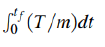
In three chosen scenarios, numerically almost matching values of Δv and the propellant mass, mp were obtained. As the flight time increases in the scenario 1, 2 and 3, Δ_v and the propellant mass (m_p) decreased. Thus, the fuel consumption could be more saved in the longer flight time and smaller input power.

Table 3: Comparisons of the optimization solutions for scenario 1, 2 and 3.

Conclusion

In this paper, minimum-fuel, low-thrust Earth-to-Mars trajectory optimization in the heliocentric two-dimensional polar coordinate system for the spacecraft with constant specific impulse engine have been studied. For the solutions of the optimal control problem, a well-defined TPBVP was derived as an indirect method and GPOPS-II with NLP solver, SNOPT was employed to solve the same problem as a direct method without a derivation of the TPBVP. Three Earth-to-Mars orbit transfer scenarios with different flight time and input powers were chosen to verify minimum-fuel, low-thrust trajectory optimization using both the direct method and the indirect method. Numerically matching optimization results were obtained by both methods with the same on-off-on thrust sequence where the primer vector theory holds. The results are useful for broad trajectory search using the CSI engine in the preliminary phase of mission designs.

Acknowledgement

This work was supported by the National Research Foundation of Korea (NRF) Grant Funded by the Ministry of Science and ICT (NRF-2017R1A5A1015311).

Conflict of Interest Statement

The author declares that I have no conflict of interests.

References

1. Rayman MD, Williams SN. Design of the first interplanetary solar electric propulsion mission. J Spacecr Rockets. 2002;39(4):589-595.

   [Crossref] [Google Scholar]

2. Rayman MD, Fraschetti TC, Raymond CA, Russell CT. Dawn: A mission in development for exploration of main belt asteroids Vesta and Ceres. Acta Astronautica. 2006;58(11):605-616.

   [Crossref] [Google Scholar]

3. Kugelberg J, Bodin P, Persson S, Rathsman P. Accommodating electric propulsion on SMART-1. Acta Astronautica. 2004;55(2):121-130.

   [Crossref] [Google Scholar]

4. Nishiyama K, Hosoda S, Ueno K, Tsukizaki R, Kuninaka H. Development and testing of the Hayabusa2 ion engine system. Trans JSASS Aerospace Tech Japan. 2016;1430:131–140.

   [Crossref] [Google Scholar]

5. Taheri E, Li NI, Kolmanovsky I. Co-state initialization for the minimum-time low-thrust trajectory optimization. Adv Space Res. 2017;59(9):2360–2373.

   [Crossref] [Google Scholar]

6. Morante D, Rivo MS, Soler M. A survey on low-thrust trajectory optimization approaches. Aerospace 2021;8(3):1-39.

   [Crossref] [Google Scholar]

7. Von Stryk O, Bulirsch R. Direct and indirect methods for trajectory optimization. Ann Oper Res. 1992;37:357-373.

   [Crossref] [Google Scholar]

8. Vadali SR, Nah R. Fuel-optimal planar Earth–Mars trajectories using low-thrust exhaust-modulated propulsion. J Guid Control Dyn. 2000;23(3):476–482.

   [Crossref]

9. Jiang F, Baoyin H, Li J. Practical techniques for low-thrust trajectory optimization with homotopic approach. J Guid Control Dyn. 2012;35(1):245–258.

   [Crossref] [Google Scholar]

10. Zhang Z, Gong S, Li J. The fuel-optimal trajectory for finite-thrust LUNAR ASCENT. Aerospace Sci Technol. 2014;39:675–684.

    [Crossref] [Google Scholar]

11. You L, Dong Y, Zhaowei S. Time efficient sliding mode controller based on Bang–Bang logic for satellite attitude control. Aerospace Sci and Technol. 2018;75:342–352.

    [Crossref] [Google Scholar]

12. Chi Z, Wu D, Jiang F, Li J. Optimization of variable-specific-impulse gravity-assist trajectories. J Spacecr and Rocket. 2020;57( 2):1-9.

    [Google Scholar]

13. Zhu Z, Gan Q, XinYang, Gao Y. Solving fuel-optimal low-thrust orbital transfers with bang-bang control using a novel continuation technique. Acta Astronautica. 2018;137:98–113.

    [Crossref] [Google Scholar]

14. Tang S, Conway BA. Optimization of low-thrust interplanetary trajectories using collocation and nonlinear programming. J Guid Control Dyn. 1997;18(3):247–262.

    [Crossref] [Google Scholar]

15. Kluever CA. Optimal low-thrust interplanetary trajectories by direct method techniques. J Astronaut Sci. 1997;45(3):247–262.

    [Crossref] [Google Scholar]

16. Patterson MA, Rao AV. Exploiting sparsity in direct collocation Pseudospectral methods for solving optimal control problems. J Guid Control Dyn. 2012;49(2):364–377.

    [Crossref] [Google Scholar]

17. Bryson JAE, Ho YC. Applied Optimal Control: Optimization, Estimation and Control, 1975.
18. Guo Y, Feng D, Wang X, Li C, Liu Y. The Earth-Mars transfer trajectory optimization of solar sail based on hp-adaptive pseudospectral method. Discrete Dyn Nat Soc. 2018;1–14.

    [Crossref] [Google Scholar]

19. Patterson MA, Rao AV. GPOPS-II: A MATLAB software for solving multiple-phase optimal control problems using hp-adaptive Gaussian quadrature collocation methods and sparse nonlinear programming. ACM Trans Math Softw. 2014;41(1):1–37.

    [Crossref] [Google Scholar]

20. Topputo F, Zhang C. Survey of direct transcription for low-thrust space trajectory optimization with applications. Abstr Appl Anal. 2014;851720:1–15.

    [Crossref] [Google Scholar]

21. Conway BA. Spacecraft Trajectory Optimization. Cambridge, 2010, pp. 16–24.
22. Geering HP. Optimal control with engineering applications, 2007.
23. Gill PE, Murray W, Saunders MA. SNOPT: An SQP algorithm for large-scale constrained optimization. SIAM Rev. 2005;47(1):99–131.

    [Crossref] [Google Scholar]

24. Darby CL, Hager, WW, Rao AV. Direct trajectory optimization using a variable low-order adaptive pseudospectral method. JSpacecr Rocket, 2011;48(3):433–445.

    [Crossref] [Google Scholar]