Journal of Antivirals & Antiretrovirals
Open Access
ISSN: 1948-5964
ISSN: 1948-5964
Research Article - (2021)
In this paper, the Markov Chain Monte Carlo (MCMC) method is used to estimate the parameters of Logistic distribution, and this method is used to classify the credit risk levels of bank customers. OpenBUGS is bayesian analysis software based on MCMC method. This paper uses OpenBUGS software to give the bayesian estimation of the parameters of binomial logistic regression model and its corresponding confidence interval. The data used in this paper includes the values of 20 variables that may be related to the overdue credit of 1000 customers. First, the "Boruta" method is adopted to screen the quantitative indicators that have a significant impact on the overdue risk, and then the optimal segmentation method is used for subsection processing. Next, we filter three most useful qualitative variables. According to the WOE and IV value, and treated as one hot variable. Finally, 10 variables were selected, and OpenBU-GS has been used to estimate the parameters of all variables. We can draw the following conclusions from the results: customer’s credit history and existing state of the checking account have the greatest impact on a customer's delinquent risk, the bank should pay more attention to these two aspects when evaluating the risk level of the customer.
Data analysis; Monte Carlo model; OpenBUGS; Overdue risk
The Markov Chain Monte Carlo method (MCMC), originated in the early 1950s, is a Monte Carlo method that is simulated by computer under the framework of Bayesian theory. This method introduces Markov process into Monte Carlo simulation, and achieves dynamic simulation in which the sampling distribution changes as the simulation progresses, which makes up for the shortcoming that traditional Monte Carlo integral can only simulate statically. MCMC is a simple and effective computing method, which is widely used in many fields, such as statistics, Bayes problems, computer problems and so on. Credit business also known as credit assets or loan business, which is the most important asset business of commercial Banks. By lending money, the principal and interest are recovered, and profits are obtained after deducting costs. Therefore, credit is the main means of profit for commercial Banks.
By expanding the loan scale, the bank can bring more income, and inject more power into the social economy, so that the economy can develop faster and better.
However, with the expansion of credit scale, it is often accompanied by risks such as overdue credit. Banks can reduce credit overdue risk from two aspects, one way is to increase the credit overdue penalties, such as lowering the personal credit, dragging into the blacklist, and so on with the rapid development of Internet personal credit registry has more and more influence on the individual. A bad credit report will bring much inconvenience for the individual, so, in order to avoid the adverse impact on your credit report, borrowers tend to repay the loan on time, but these means are all belong to afterwards, although reduced the frequency of overdue frequency, but still caused a certain loss to the bank.
Selectively lending to "quality customers" can reduce Banks' credit costs even more if they anticipate the likelihood of delinquency in advance, before the customer takes out the loan. How to identify whether the client is the "good customer" will need to collect overdue related information about the customer in advance, through the establishment of probability model between relevant variables and overdue, thus to rank the customer's risk grade of overdue, if customers risk level is extremely high, the bank should choose to increase loan interest or refuse to reduce the risk of credit bank loans [1].
This paper includes the following three parts: model introduction and data description, data preprocessing and OpenBUGS simulation and summary.
Overview of logistic model
If we want to use linear regression algorithm to solve the problem of a classification, (for classification, y value equal to 0 or 1), but if you are using the linear regression, then assumes that the function of the output value may be greater than 1, or much less than zero, even if all the training sample label y is 0 or 1 but if algorithms get value is greater than 1 or far less than zero, will feel very strange.
So the algorithm we're going to study in the next section is called the logistic regression algorithm, and this algorithm has the property that its output value is always between 0 and 1. So, logistic regression is a classification algorithm whose output is always between 0 and 1.
First, let's take a look at the LR of the dichotomy. The specific method is to map the regression value of each point to between 0 and 1 by using the SIGmoid function shown in Figure 1.

Figure 1: Sigmoid function.
As shown in the figure, let z=w.x+b, when z>0, the greater z is, the closer the sigmoid returns to 1 (but never more than 1). On the contrary, when z<0, the smaller z is, the closer the sigmoid return value is to 0 (but never less than 0).
This means that when you have a binary classification task (positive cases corresponding labeled 1, counter example corresponding labels 0 and samples of each of the sample space for linear regression z=w.x+b, then the mapping using sigmoid function of g=sigmoid (z), and finally output the corresponding class label each sample (all value between 0 and the one greater than 0.5 is marked as positive example), then, two classification is completed. The final output can actually be regarded as the probability that the sample points belong to the positive example after the model calculation.
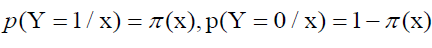
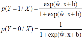
Thus, we can define the general model of the dichotomous LR as follows:
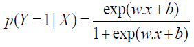
For a given input x, p(Y=1/X) and p(Y=0/X) can be obtained, and the instance x will be classified into the category with high probability value.
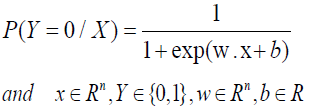
Odds of an event refer to the ratio between the probability of its occurrence and the probability of its non-occurrence. If the probability of its occurrence is P, the probability of the event is P/ (1-P), and the log odds or logit function of the event is
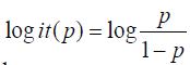
logistic regression can be obtained
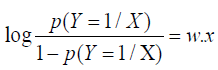
That is, the logarithmic probability of output Y=1 in the logistic regression model is a linear function of input X.
When learning logistic regression models, for a given data set
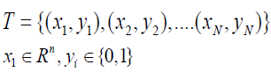
The maximum likelihood estimation method can be used to estimate the model parameters, and then the logistic regression model can be obtained set
The likelihood function is
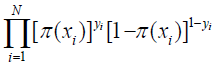
The logarithmic likelihood function is
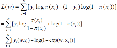
By gradient descent algorithm and newton method can get the maximum value in the L(w) and the estimates of w : wˆ then the logistic regression model
MCMC
The formula of Markov Chain is as follows
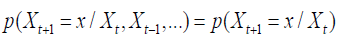
That is, the state transition probability value is only related to the current state. Let P be the transition probability matrix, where pij represents the probability of the transition from i to j. So we can prove that
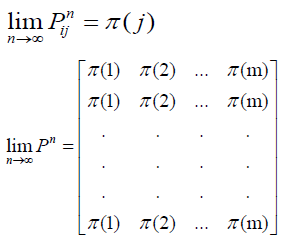
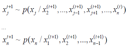
Where π is the solution to πP=π. Since the probability of x obeys π(x) after each transfer, it is possible to sample from π (x) by transferring the different bases to this probability matrix. Then, given π (x), we can construct the transition probability matrix by the Gibbs algorithm.
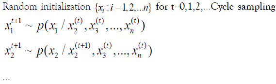
Gibbs algorithm
Data description and preprocessing
The German credit card data set is adopted in this paper, which contains 20 variables, including 7 quantitative variables and 13 qualitative variables. The details are shown in Table 1.
| Quantitative variable | Qualitative variable | |
|---|---|---|
| Duration | Purpose | Property |
| Credit amount | Credit history | Housing |
| Installment rate | Checking account status | Other installment plans |
| Present residence | Savings | Job |
| Age | Other debtors | Telephone |
| Existing credits | Personal | Foreign worker |
| People liable | Present employment | |
Table 1: Data specification.
The data set includes 20 variables, the influence of different variables on credit overdue is different, adopting too many variables will not only increase the cost of collecting data, and waste customer’s, also increases the complexity of the model, reduce the accuracy of prediction, so before to fitting the model we need to screen all the indicators which have a significant effect. The following content will be introduced from the screening of quantitative indicators and the screening of qualitative indicators.
“Boruta” screening of quantitative indicators
The goal of Boruta is to select all feature sets related to dependent variables, which can help us understand the influencing factors of dependent variables more comprehensively, so as to conduct feature selection in a better and more efficient way.
Algorithm process:
1. Shuffle the values of various features of feature matrix X, and combine the post-shuffle features and the original real features to form a new feature matrix.
2. Using the new feature matrix as input, training can output the feature importance model.
3. Calculate Zscore of real feature and shadow feature.
4. Find the maximum Zscore in the shadow features and mark it as Zmax.
5. The real feature whose Zscore is greater than Zmax is marked as "important", the real feature whose Zscore is significantly less than Zmax is marked as "unimportant", and is permanently removed from the feature set.
6. Delete all shadow features.
7. Repeat 1 to 6 times until all features are marked as "important" or "unimportant" The importance order of quantitative variables using the Boruta package of R software is shown in Figure 2.

Figure 2: Quantitative variable importance.
The first three quantitative variables duration, create amount and age were selected into the model in order of importance, and the continuous variables were divided into boxes, with WOE (weight of evidence) and IV (Importance Value) values dividing the variables with the best predictive ability into groups
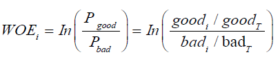
Where good stands for the number of good tags in each group, goodT for the total number of good tags; The same for bad.
Where N is the number of grouped groups, and IV can be used to represent the grouping ability of a variable, as shown in Table 2.
| IV | Strength |
|---|---|
| <0.03 | Extremely low |
| 0.03-0.09 | Low |
| 0.1-0.29 | Medium |
| 0.3-0.49 | High |
| >0.5 | Extreme high |
Table 2: IV vs. ability to predict.
To make the difference between groups as large as possible, smbinning package in R software is used to segment the continuous variable duration, credit amount and age using the optimal segmenting method. The result of segmenting is shown in Figure 3.

Figure 3: Optimal segmentation of continuous variables.
The Duration loan variable was divided into three sections: [0,11], (11,33) and (33,+∞); Credit amount loan amount (a continuous variable) was divided into four paragraphs: [0,3446] and (3446,3913], (3913,7824], (7824,+∞]; The Age of the Age applicant is divided into [0,25] and (25,+∞). All segments of the variable are corresponding to the WOE value with a large difference, indicating a large difference between groups. The IV value calculated according to the WOE value of the group are respectively duration: 0.225, Credit amount: 0.229, age: 0.073.
Screening of qualitative indicators
IV values were calculated for all types of variables and sorted from high to low. Since the data only contained 1000 rows and the sample size was relatively small, only variables with large IV values, namely those with obvious classification effect, were selected in this paper. Three variables with IV values greater than 0.15 were selected and the results were shown in Table 3.
| Vars | IV |
|---|---|
| Account status | 0.666 |
| Credit history | 0.2932 |
| Savings | 0.196 |
Table 3: Screening of qualitative indicators
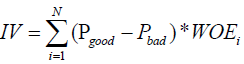
For each of the three selected qualitative indicators, the possible values of the variables are matched to a 0-1 variable. For example, the variables checking account status are treated as
variables A11, A12, A13, and A14,Variables may have values as shown in the Table 4.
| Vars | Accuracy rate |
|---|---|
| Account status | A11,A12,A13,A14 |
| Credit history | A30,A31,A32,A33,A34 |
| Savings | A61,A62,A63,A64,A65 |
Table 4: Variables values.
Step forward likelihood ratio test
After preprocessing, there are 17 variables, not all of which have significant influence on the overdue risk. Before fitting the model, variables with small correlation and more significant significance are screened out, this can not only improve the classification accuracy of the model, but also simplify the model and reduce the cost of collecting customer information for Banks [2].
Variables with significant influence on overdue risk were selected by using the forward likelihood ratio test. The simulation results of SPSS are shown in Table 5.
| Vars | LL | -2LL Change | DF | Sig. |
|---|---|---|---|---|
| A12 | -500.591 | 4.05 | 1 | 0.044 |
| A14 | -531.725 | 66.318 | 1 | 0 |
| A13 | -503.329 | 9.526 | 1 | 0.002 |
| A21 | -515.948 | 34.765 | 1 | 0 |
| A34 | -503.507 | 9.882 | 1 | 0.002 |
| A30 | -501.945 | 6.758 | 1 | 0.009 |
| A31 | -503.137 | 9.141 | 1 | 0.002 |
| A61 | -506.506 | 15.879 | 1 | 0 |
| A62 | -500.883 | 4.634 | 1 | 0.031 |
| A131 | -501.842 | 6.551 | 1 | 0.01 |
Table 5: Step forward likelihood ratio test result.
Model training and prediction
The significance level was set as 0.05. A total of 10 variables were screened to establish the model:

Where β0 is the constant term, β1 (i =1,2,...,10) is the partial regression coefficient of independent variable;
Parameters of the model have been given independent "non-noninformative" prior distribution, and OpenBUGS software is used for modeling and sampling, as well as Doodle modeling through OpenBUGS, to specify the distribution type and logical relationship of various parameters, as shown in the Figure 4.

Figure 4: Doodle model.
Each ovals represent a node IN the graph, rectangle with constant node, single arrow from the parent node to the random child nodes, hollow double arrows indicate the parent node to the logical type child nodes, the rectangular outside for tablet, the lower left corner "for (I IN 1: N)" said for loop, is used to calculate the likelihood function of all samples, and the overall likelihood function is obtained [3].
The posterior distribution statistics for each parameter were obtained using OpenBUGS software, as shown in Table 6.
| Mean | SD | MC error | Val2.5pc | Median | Val97.5pc | Start | Sample | |
|---|---|---|---|---|---|---|---|---|
| beta0 | -1.715 | 0.5688 | 0.0077 | -2.806 | -1.732 | -0.6263 | 1001 | 10000 |
| beta1 | -0.422 | 0.0409 | 0.0022 | -0.8879 | -0.4183 | -0.0158 | 1001 | 10000 |
| beta2 | -1.584 | 0.0363 | 0.0022 | -2.086 | -1.578 | -1.1 | 1001 | 10000 |
| beta3 | -0.7002 | 0.0598 | 0.0025 | -1.637 | -0.6884 | -0.1802 | 1001 | 10000 |
| beta4 | 0.8689 | 0.0218 | 0.0019 | 0.5103 | 0.8637 | 1.233 | 1001 | 10000 |
| beta5 | -0.7936 | 0.0286 | 0.0009 | -1.266 | -0.7879 | -0.3396 | 1001 | 10000 |
| beta6 | 0.8922 | 0.0759 | 0.0017 | -0.2776 | 0.8786 | 2.149 | 1001 | 10000 |
| beta7 | 1.656 | 0.0703 | 0.002 | 0.0646 | 1.585 | 3.672 | 1001 | 10000 |
| beta8 | 0.6818 | 0.0285 | 0.0015 | 0.2262 | 0.6755 | 1.146 | 1001 | 10000 |
| beta9 | 0.5608 | 0.0466 | 0.0016 | -0.1907 | 0.5603 | 1.32 | 1001 | 10000 |
| beta10 | -0.3846 | 0.0309 | 0.0029 | -0.8548 | -0.3755 | 0.0714 | 1001 | 10000 |
| tau | 270.9 | 0.0062 | 0 | 5.065 | 105 | 1524 | 1001 | 10000 |
Table 6: Parameter estimation result of MCMC.
Where, MC error represents the error of Monte Carlo simulation and is used to measure the variance of the mean value of parameters caused by simulation.Val2.5 PC and VAL97.5 PC represent the lower and upper limits of the 95% confidence interval of the median, respectively; Median is usually more stable than mean; Start represents the starting point of Gibbs sampling. In order to eliminate the influence of initial value on sampling, sampling is started after 1001 times. Sample represents the total number of samples extracted. A total of 10,000 samples were extracted in this paper [4].
According to the parameters of Bayesian estimation, the error of model Colot simulation is generally relatively small, which indicates that the model has a good effect. With each parameter of the Gibbs sampling sample mean as a parameter to estimate, from the point of the results, the variable whether checking account status values for A13 (greater than 200 DM) and A14 (no checking account), variable credit history whether values for A30 (not credit) and A31 (have to pay all the bank's credits) have bigger influence on the overdue risk, relative variable savings for A61 values (<100 DM) and A62 (100<x<500 DM) has little impact on the overdue risk, indicating that the customer's historical credit history and the current check status have a greater impact on the overdue risk, that is, the customer's historical credit and current economic status have a greater impact on the overdue risk. Banks should focus on these two aspects when judging the customer's credit risk level [5].
The logistic regression equation can be obtained
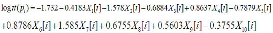
When dividing the overdue risk level of customers, there may be two wrong divisions, that is, dividing "high-quality customers" into high-risk customers and high-risk customers into "high-quality customers". Generally speaking, the economic costs of these two wrong divisions are different. For Banks, the cost matrix is shown in the Table 7 (0=Good, 1=Bad) (Table 7) [6].
| 0 | 1 | |
| 0 | 0 | 1 |
| 1 | 5 | 0 |
Table 7: Cost matrix.
The rows represent the actual classification and the columns the predicted classification. It is worse to class a customer as good when they are bad (cost=5), than it is to class a customer as bad when they are good (cost=1). Define the loss function as
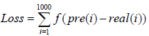
pre(i) and real(i) is The classification results of the ith sample and the actual category, respectively, and f(x) is a piecewise function:
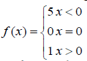
Each sample input the results of logistic regression model as a probability value, if the probability value is greater than a given probability value is the sample classification is 1, otherwise the classification of 0, due to the loss of the two types of error, according to the different probability of loss matrix can be calculated at a given value under the condition of overall losses, the results as shown. It can be seen that when the given probability value is 0.21, the overall loss is the smallest. The Confusion matrix is shown in the Table 8. The precision of the model is 85%. The model identifies the vast majority of high-risk customers (Figure 5 and Table 8).

Figure 5: Loss diagram.
| 0 | 1 | |
| 0 | 513 | 187 |
| 1 | 45 | 255 |
Table 8: Confusion matrix.
Figures 6-8 shows the iteration history diagram, autocorrelation function diagram and kernel density diagram of all parameters.

Figure 6: Iteration history of OpenBUGS.

Figure 7: The autocorrelation diagram of OpenBUGS.

Figure 8: The nuclear density of OpenBUGS.
Monte Carlo simulation starts from the initial value given for each parameter. Due to the randomness of extraction, the first part of extracted value is used as an independent sample obtained by annealing algorithm. Therefore, we must judge the convergence of the extracted Markov Chain. The convergence of Markov chains can be analyzed according to the results of parameter extraction [7].
Iteration history diagram: From the graphs in Figure 5 we can safely conclude that the chains have converged as the plots exhibits no extended increasing or decreasing trends, rather it looks like a horizontal band.
Nuclear density figure: According to the distribution density of extracted samples, it can be seen that the samples extracted by Gibbs algorithm are mostly concentrated in a small area, which can also explain the convergence of Markov chain [8].
Autocorrelation diagram: Autocorrelation plots clearly indicate that the chains are not at all auto correlated. The later part is better since samples from the posterior distribution contained more information about the parameters than the succeeding draws. Almost negligible correlation is witnessed from the graphs in Figure 6. So the samples may be considered as independent samples from the target distribution i.e. the posterior distribution [9,10].
This paper constructs a binomial logistic regression model based on the customer characteristic data of Banks.
Content mainly includes two parts, the first is the part of data pretreatment, the original data contains 20 variables, in order to make the model more concise, and improve the accuracy of classification model, reduce the cost of information collection and the time cost of customers, using "Boruta" method of screening of three quantitative indicators, and use the optimal segmentation method will be treated as continuous variable section.
Then, three qualitative variables were selected into the model by calculating the IV value of the variable, and the qualitative variables were treated with a unique heat type.
Two logIST-IC regression of SPSS software was used to screen out 10 variables with significance less than 0.05 into the model.
All the selected variables were brought into OpenBUGS software to obtain the parameter Bayesian estimation of the binomial logistic regression model. From the estimation results, it can be seen that the customer's historical credit (Credit history) and current economic status (Checking account status) have the greatest impact on credit delinquency. Banks should pay more attention to these two aspects when evaluating the customer's credit risk level.
We have no conflict of interests to disclose and the manuscript has been read and approved by all named authors.
This work was supported by the Philosophical and Social Sciences Research Project of Hubei Education Department (19Y049), and the Staring Research Foundation for the Ph.D. of Hubei University of Technology (BSQD 2019054), Hubei Province, China.
Citation: Zhao B, Cao J (2021) Logistic Model of Credit Risk Based on MCMC Method. J Antivir Antiretrovir. S18:001.
Received: 22-Feb-2021 Accepted: 08-Mar-2021 Published: 15-Mar-2021 , DOI: 10.35248/1948-5964.21.s18.001
Copyright: © 2021 Zhao B, et al. This is an open-access article distributed under the terms of the Creative Commons Attribution License, which permits unrestricted use, distribution, and reproduction in any medium, provided the original author and source are credited.