Journal of Geography & Natural Disasters
Open Access
ISSN: 2167-0587
ISSN: 2167-0587
Research Article - (2017) Volume 7, Issue 1
In line with Climate change rainfall seasonal fluctuation and rainfall amount have major impact on flood and becoming a trait to human life and properties especially on agriculture and different installation. Therefore estimating the runoff and identifying flood prone area at different return period is very essential for effective flood mitigation measure. One of the possible approaches for identifying flood prone area is use of integration of RS with hydraulic models (HECRAS). The present study area is of Woybo River catchment, south western Ethiopia, Shuttle Radar Topography Mission (SRTM) Digital Elevation Model (DEM), 90 m resolution downloaded from united states geological survey, were used to extract the river geometry. Daily peak rainfall data from tow metrological stations (1990-2013), collected from national metrological agency, were used for estimating design rainfall and runoff for 5, 10, 25, 50, 100 and 200 return period. In HEC-RAS, river geometry, boundary conditions, manning’s n value of different land cover, designed runoff for different return periods were inputted then steady flow analysis was carried out. estimated design rainfall frequency showed expected peak rainfall were 63.2, 70.87, 80.57, 87.77, 94.91 and 102.02 mm and estimated design runoff were 378, 461, 568, 650.5, 733, and 817 m3/se. Steady analysis showed that water surface elevation in the longitudinal profile increase with increasing return period, Inundation area were 1727, 1788, 18560, 1905, 1950 and 1987 ha respectively. The study also suggested that flood prone areas were at the lower reach along the banks of the river extending to 50 m right and left. The finding has been used for planning and decision making in insuring that this areas are protected and limit the risk of damage occurring.
Keywords: Design rainfall, Design runoff, RS and HEC-RAS
Flooding is the most common and most spatially distributed natural hazard across the world, and every year it cause considerable damage [1]. It annually causes great deal of human and financial losses [2]. These losses include destruction of agricultural soils, devastation of different installations [3]. According to Abhas and Jessica [4], flood affected 178 million people Worldwide in 2010 alone and has resulted in a total financial loss in the exceptional years such as 1998 and 2010 exceeded $40 billion. Flood is the most devastating natural hazards in Africa that causing loss of lives caused by tropical cyclones and severe storms. It primarily caused by abnormally high rainfall (e.g., due to tropical cyclones) as well as a number of human-induced contributory causes. It is also the second major natural hazard next to drought in Ethiopia [5]. It is mainly linked with the national topography of the highland mountains and lowland plains with natural drainage systems formed by the principal river basins [6]. The country received about 80% of the rains in rainy season concentrated in the three months between June and September. During this season the major perennial rivers as well as their numerous tributaries forming the country’s drainage systems which originate from the centrally situated highlands and make their way down to the peripheral or outlying lowlands carry their peak discharges [7]. Torrential down pours are common in most parts of the country. As the topography of the country is rather rugged with distinctly defined watercourses, large scale flooding is rare and limited to the lowland areas where major rivers cross to neighbouring countries [8]. However, intense rainfall in the highlands could cause flooding of settlements close to any stretch of river course [9]. This flood cause damage crops and distraction of agricultural soil temporarily displace peoples from their usual doweling, death of organisms and precious human life, distraction of constrictions such as brigs, power and telecom lines, roads etc. in various parts of the country. According to the EM-DAT 2008 report on disaster risk Management Programs for Priority Countries Africa, major floods in Ethiopia from 1999-2009 affected 1,108604 people. In the last few decades the frequency and magnitude of flood in the country have increased rapidly as a result of climate change as well as land-use change [10]. While the damage intensifying with increasing population due to increasing land and forest degradation, encroachment of people to settle in close proximity to the flood prone areas [11]. Also activities in the catchment such as land clearing for agriculture may increase the magnitude of flood which increases the damage to the properties and life [12]. Were as its intensity and return period generally are affected by volume and time of upstream surface runoff and river or flood conditions, physical characteristics of watershed (area, morphology), hydrological characteristics of the watershed (rainfall, storage, evapo-transpiration), and human activities causing and intensifying the flood flows [13].
Although, flood is normally expected in Ethiopia studies are conducting on flood Inundation Area Mapping in some parts of the country using GIS and RS to facilitate the administrators and planners for flood hazard mitigation measure but thus studies not integrate hydrological and hydraulic models. However, the identification of flood-prone areas through integrating remote sensing and hydraulic models are not well studied. For instance Getahun and Gebre [14], used integration of GIS and one dimensional hydraulic model for Flood Hazard Assessment and Mapping of Flood Inundation Area from stream flow data of the Awash River Basin in Ethiopia. Also flood is a common occurrence in Woybo River catchment, where the current study is carried out. So far, there were no studies on the problem so as to sustainably manage the catchment. This study was, therefore, very important to identify flood prone areas of the catchment from daily peak rainfall data those delineate 5, 10, 25, 50, 100 and 200-years flood for planning and decision making while insuring that this areas are protected from flooding and to limit the risk of damage occurring.
Description of the study area
The study was conducted at Woybo river catchment. Woybo River is one of the main tributaries of the Omo Gibe Basin. It is found in north east of the basin in South western, Ethiopia. The location of the basin lies between 6° 55' 20" N to 7° 2' 40" N latitude and 37° 51' 40" to 37° 31' 0"E longitudes, as in Figure 1. The catchment area of the study area is 561.26 km2.

Figure 1: Location of Woybo River catchment, (own processing).
Topographic characteristics
The topography of Woybo river catchment is very steep in upper reaches and sudden in lower reaches, as in Figure 2. The altitude ranges from 768 to 2946 m.a.s.l. The mean elevation is 1911 m.a.l and with a standard devotion of 579.47.

Figure 2: Digital elevation model.
According to Gizachew [15] slope classification the vast area 48.91% (274.52 km2) of the study area have the topography characteristics feature of flat terrain which lies within slope ranges from 0-3% and 0.16% (0.96 km2) are mountainous terrain which lies within the slope range of >50 % , as in Figure 3.

Figure 3: Slope classification.
Drainage
The drainage network of Woybo river catchment extracted From SRTM DEM 90 m. The river catchment contains 23 streams with reference to Strahler [16] a total length of 148.9 km and a Longest flow path length (LFPL) of 1944 km with reference Horton [17] also a bifurcation ratio of 0.96 with reference to Horton [18] and Strahler [19], the river catchment is third order and a drainage density of the entire catchment is 0.45 km/km2.
Soils
The soil types in an area are important as they control the amount of water that can infiltrate into the soil, and hence the amount of water which becomes runoff. The major soil in Woybo river catchment according to the international soil classification method, (FAO, 1998) are dystric Nitosols (55.3%), pellic vertisols (31.94%), Chromic Luvisols (10.54%) and Eutric cambisols (1.69%), as in Figure 4.

Figure 4: Soil classification map
Climate
The study area has tropical climate regime. Monthly average temperature of the study area varies between 21.5°C in Mar to 17.8°C July. Monthly average relative humidity (RH) of Woybo river catchment falls in the class of 44.61-76.65% and the average sunshine hour for almost 8 months of a year is about 80%, and falls below 50% during monsoon. Rainfall distribution of the study area as part of the south region is largely controlled by the South-North movement of the Inter Tropical Convergence Zone (ITCZ) [20]. The study area is characterized by bimodal rain fall type, short rainy season, which extends between March and May and locally known as “Belg” receives 28% (338.4 mm) and the long rainy season and locally known as Kiremt, which extends from June up to October (kerempt) receive 62 % (847.9 mm). The average annual rainfall of the study period 1990 to 2013 is 1366 mm. Rainfall play a vital role with respect to flood threat within the study area and with most threatening events between Julys to September 55% of the annual rains fall during the months.
Methodology
In this research the Storm water Management and Design Aid (SMADA) distribution model, Rainfall runoff generation SCS hydrology model and HEC-Geo-RAS and HEC RAS were used. The methods followed in this study are schematically represented in Figure 5.

Figure 5: Flow chart for peak runoff estimation.
Image classification
Before image classification was done, actual field observation was held and a total of eight classes were selected which include cropland, forest, shrubs land, bush land grazing land, bare lands, woodland and Built-up Land sat 7 imagery (path 169 and row 55) of the period march 2013 was used to classify the current land cover of the study area. The land cover classification was done in Arc GIS 10 and ERDAS 9.2 software’s. In Pre-processing of image classification extraction and image staking were done using band combination in Arc-GIS to form different combination of Red, Green, Blue colour composition. The basic bands 4, 3 and 2 were used prior to classification to improve visualization of the image for the prospected classification [21].
Post Image classification
This research used supervised image classification to classify the dominant land cover types in the study area using reference sources imagery or field notes [22]. Visual image interpretation was done to the land sat 7 image using supervised image classification in ERDAS 9.2. Four stages were carried out to classify the land cover types as Training site selection and sampling intersect were performed, Signature analyses of each land cover types were done, Supervised classifications of data set were performed based on maximum likelihood classifier. Maximum likelihood classifier (MLC) is the most widely adopted parametric classification algorithm for land cover information [23], and finally land cover types in the study are classified and mapped.
Accuracy assessment
Accuracy assessment was done after the image has been classified in to different land use classes based on their pixel value or brightness value [24], after the classified image has been produced its quality was assessed using ground truth [25]. For the accuracy assessment a total of 430 ground truth points 36, 180, 43, 60, 32, 24, 30 and 34 from shrub land, cropland land, woodland, bush land, Built-up, forest, grazing land and bare lands respectively, was used for accuracy assessment to quantitatively determine how effectively pixels were grouped into the correct feature classes.
Daily peak rainfall, design flood frequency and return period analysis
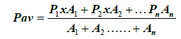
The Point gauged Daily rainfall data of 23 years (1990-2013) from two representative Meteorological stations of the study area, Areka and Wolayita sodo were obtained from National Metrological Agency of Ethiopia. The data were analyzed to determine the annual daily peak rain fall of the study area using Thiessen polygon method (Equation 1):
Thiessen polygon method
In this method the rainfall recorded at each station is given a weight age on the basis of areas enclosed by bisectors around each station. The sum of the weights is one.
 (1)
(1)
Where; P1, P2…Pi are the rainfall magnitudes recorded by the stations 1, 2…i respectively, and A1, A2, A3… Ai is the respective area of the Thiessen polygons [26].
Design frequency analysis using frequency factor
The objective of frequency analysis is to relate the magnitude of extreme events to their frequency of occurrence through the use of probability distributions. The current was used six probability distributions function, Norma l, 2 parameter log normal, parameter log normal, Pearson distribution, person type III and Gambel in combination with Weibull plotting position in SMADA (storm water Design Aid) software using DISTRIB 2.0 component to estimate the expected values at different return periods of 5, 15, 25, 50, 100 and 200 years.
Testing the goodness of fit of probability distribution
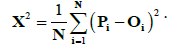
In determining the best fit distributions for design rainfall frequency for Woybo River catchment, Weibull plotting positions and thus probability distributions were plotted against the daily maximum rainfall of the river. Furthermore, the best probability distribution function was determined by comparing Chi-square values obtained from each distribution and selecting the function that gave smallest chisquare value [27], and mean square errors (RMSE) that gave smallest error. The chi-square test statistic is given by the equation.
 (2)
(2)
Where, Oil is the observed rainfall,
Eli is the expected rainfall and will have chi-square distribution with (N - k -1) degree of freedom (d.f.).
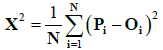 (3)
(3)
Where P is the predicted value, O is the observed value and N is the number of data.
Hydrological soil group map
Infiltration rates of soils vary widely and are affected by subsurface permeability as well as surface intake rates [28]. Soils are classified into four HSG’s (A, B, C, and D) according to their minimum infiltration rate. The different soil textures of Woybo river catchment were obtained from the digital soil and terrain database of east Africa (sea) FAO 1997. Based on the rules of hydrologic soil group classifications developed by the US Natural Resource Conservation Service (NRCS), the hydrologic soil map of Woybo river catchment was generated as shown in Figure 6. The hydrologic soil group of Woybo river catchment corresponds to the soil class are C and D, 99% of the catchment is under HSG D (clay) having highest runoff potential. It Includes clays of high swelling percent, and sub horizons near the surface and the rest 1% are C (clay loam).

Figure 6: Hydrologic soil groups map.
The curve number (CN)
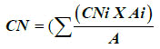
The CN is a number developed by the soil conservation service to assist in the estimation of infiltration during rainfall events. The CN is always less than 100. High curve numbers (>90) represents little or no infiltration, whereas low curve numbers (<50) represents very pervious surface. The CN was created by intersecting two shape files; the soil hydrologic group map and the land use map. Then from standard SCS-CN look up table the correct curve numbers was assigned for all the combinations. The weighted hydrologic curve number was determined for the whole Woybo river catchment area based on the three antecedent moisture conditions.
 (4)
(4)
Where: CN = weighted curve number, CNi = curve number from 1 to any no. N, Ai = area with curve number CNi, A = the total area of the Woybo river catchment.
Design peak run off estimation
The Rainfall runoff generation SCS hydrology model [29], has been used to estimate design runoff. The model inputs design rainfall of different period, Stream Length and slope, Curve Number CN and Land use or cover Area ratio were imputed and first the direct run off was calculated using the SCS CN Method (Equation 5), then peak runoff run off hydrograph was estimated in each river Stream.
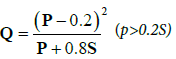 (5)
(5)
Where, S is Woybo river catchment storage (in mm); Q is the actual direct runoff (in mm); and p is the total rainfall (in mm).
The equation has one variable p and parameter s. s is related to curve number (CN) by:
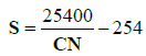 (6)
(6)
Hydraulic models used for data analysis
The current study employed the use of hydraulic models HEC-Geo- RAS 10 and HEC-RAS 4.1 models. HEC-GEORAS models was used to Creating RAS Layers under GIS environment and provide the interface between the systems, and HEC-RAS model was used to calculate water surface profiles, the methodology for hydraulic model data analysis is schematically represented in Figure 7.

Figure 7: Flow chart for flood prone area identification, (Modified from Manandhar, 2010).
Creating HEC-RAS layer
HEC-RAS Import layer was generated that are necessary to obtain the geometric simulation of the river in HEC-Geo-RAS, this HECRAS layers generated are stream centerline, flow path center lines, main channel banks, and cross-section cut lines [30] are generated using Digital Terrain Model (DTM) of the river in HEC-Geo-RAS and imported in GIS forma.
Steady flow analysis
To calculate water surface profiles in HEC-RAS, RAS GIS import file was imported to HEC-RAS which contains geometric data of the river and all the required modification, editing was done at this stage. The Manning roughness coefficient, ‘n’ value of different land resulted from field visit and calibration was inputted to HEC-RAS manning’s n value table, designed runoff of six return periods as 2, 10, 25, 50, 100 year and 200 year different periods, was inputted in steady flow data and Reach boundary conditions of Upper most cross section RS of each streams was taken as upper stream boundary and critical depth for the rest upstream and downstream was also inputted in this window. Then by running Sub critical steady flow analysis, water surface profiles were calculated. After finished simulation, HEC-RAS result cross section, longitudinal profile and Rating curve of selected reaches were visualized and RAS GIS export file was created. Finally HEC-RAS data are exported to Arc GIS using Export GIS Data button. Profile of flow was exported using export data button, which create a SDF file.
Flood inundation mapping
In Arc Map SDF file is converted into an XML file using Import RAS SDF file button imported and Stream Network, Cross Section and Bounding Polygon, Water Surface TIN and Flood inundation and flood depth mapping was generated.
Flood prone area identification
In Arc GIS Info 10 the land cover map land use map was overplayed in flood inundation and depth map using spatial analysis tool overlay to generate areas prone to flooding of the study area at different return periods.
Land cover classification
The land cover classification map for 2013 from land sat 7 images generated after running a maximum likelihood supervised classification algorithm is presented in Figure 8. The figure showed that Crop land and bush land covered for 46347.209 km2 (82.545%) and 77.435 km2 (0.137%) respectively while forest land, built up, woodland, bare land, shrubs and grazing land accounted to about 0.77 km2 (0.14%), 3.95 km2 (0.7%), 1 km2 (0.19%), 6.551 km2 (1.167%) and 1.9 km2 (0.3%) respectively. The results of classification accuracy assessment are showed an overall accuracy of 90.47% and Overall Kappa Statistics of 0.876 from the accuracy assessment report table.

Figure 8: Classified Land Cover map.
Design peak rainfall
The result of deign rainfall of 5, 10, 25, 50, 100 and 200-years Return Period for year 1990-2013 analyzed by six PDFs using SMDA software are summarized below in Table 1. Chi-square values for each PDF are estimated by using (Equation 2). Chi-square values varied from 0.12 to 0.39 for 6 PDFs. Least Chi-square values are observed in Gambel Type I distribution for prediction of design rainfall in Woybo river catchment. The chi-square values for normal, log-normal, 2 parameter log normal, Pearson type-III, log-Pearson type-III, 3 parameter log normal and Gumbel distributions are 0.21, 0.33, 0.489, 0.365, 0.39 and 0.124, and also a RMSE value of 4.48, 3.67, 3.297, 3.416, 3.313 and 3.105 respectively. Gambel combined with Weibull showed design rainfall frequency of 63.20, 70.87, 80.57, 87.77, 94.91 and 102 mm for 5, 10, 25, 50, 100 and 200 years return periods respectively, which gave minimal errors with the root mean square errors.
| Plotting Position | Error measure | Probability Distributions | |||||
|---|---|---|---|---|---|---|---|
| Normal | 2 para Log normal | Person Type III | Log person Type III | 3 para Log normal | Gambel | ||
| Weibul | Root Mean SquaredErrors (RMSE) | 4.48 | 3.67 | 3.3 | 3.42 | 3.31 | 3.11 |
| Chi-square | 0.21 | 0.33 | 0.36 | 0.49 | 0.39 | 0.12 | |
| Return period (year) | Expected Rainfall (mm) | ||||||
| 5 | 63.32 | 62.62 | 60.44 | 61.39 | 61.74 | 63.2 | |
| 10 | 68.58 | 69.05 | 68.57 | 68.32 | 68.84 | 70.87 | |
| 25 | 74.19 | 76.62 | 79.47 | 77.27 | 77.86 | 80.57 | |
| 50 | 77.82 | 81.95 | 87.86 | 84.1 | 84.62 | 87.77 | |
| 100 | 81.08 | 87.05 | 96.37 | 91.07 | 91.41 | 94.91 | |
| 200 | 84.06 | 92 | 105.02 | 98.25 | 98.29 | 102.02 | |
Table 1: Predicted frequency using six PDF.
This finding is in agreement with Bishaw, which reported that Gumbel’s method is the best fit that is; this method is with the lower Chi Square value for Meki and Ribb River. Similarly ICIMOD [31], studded Mapping Flood Hazard and Risk in a Vulnerable Terai Region: The Ratu Watershed Nepal reported that Gumbel distribution is more appropriate for the rainfall analysis. In contrast with this finding the works of Singh et al. [32], reported that log-Pearson type-III is the best probability distribution and with the works of Mandal et al. [33], which reported that Log Pearson Type III is the best fit PDF for prediction of annual rainfall but he also reported Gumbel and Log Pearson Type III distribution are best fit PDFs for prediction of monsoon and postmonsoon rainfall. The finding of this study difference might be due to data sample size.
Design runoff
The daily peak rainfall data was estimated and the weighted curve number of Woybo river catchment has been used for the estimation of direct runoff. Then the potential maximum retention (S) is easily calculated from the CN value. Therefore, S is 24.43 and or accumulated runoff depth are calculated for different return period 5, 10, 25, 50, 100 and 200 year these are 63.2, 70.8, 80.57, 87.77, 94.91 and 102.02 mm respectively which were used to estimate the deign runoff in m3/ se using Rainfall runoff generation SCS hydrology model for different return period and the result of design runoff were 378, 461, 568, 650.5, 733, and 817 m3/se. as shown in SCS hydrograph as in Figure 9a-9f respectively. Similarly Samah [34], in his study found that the average annual runoff depth for the study area (Wadi Su'd watershed) is 36.3 mm, and the average volume of runoff from the same watershed is 67840.2 m3/year.

Figure 9: Design runoff SCS hydrograph in different return period.
The design runoff Analyzed in all 23 reach of the river catchment showed that the average runoff value contributed by thus river reaches is found 4% of the catchment which is found 413.2 m3/sec, as in Table 2. Generally design runoff analyzed from thus reach of Woybo river catchment showed that upper reach’s generate an average runoff of 5879.53 m3/sec which is the large 58.6% runoff contribution and lower reach’s generate 4155 m3/sec which is 41.4% contribution to the entire river catchment.
| Woybo River Reach Name | Design runoff m3/sec | Average | Percent | |||||
|---|---|---|---|---|---|---|---|---|
| 5 y | 10 y | 25 y | 50 y | 100 y | 200 y | |||
| Woyboupper reach 10 | 166.5 | 217.1 | 282 | 330.8 | 379.9 | 429.3 | 300.93 | 3% |
| Woyboupper reach 11 | 535 | 632.5 | 745.8 | 824 | 897.8 | 968.5 | 767.26 | 8% |
| Woyboupper reach 13 | 271.7 | 336.2 | 417.2 | 476.9 | 535.9 | 594.7 | 438.76 | 5% |
| Woyboupper reach 14 | 340.2 | 410.7 | 497.8 | 561.1 | 623.2 | 684.7 | 519.61 | 5% |
| Woyboupper reach 2 | 149.5 | 192.8 | 248.3 | 289.9 | 331.5 | 373.3 | 264.21 | 3% |
| Woyboupper reach 3 | 97.9 | 129.4 | 170.4 | 201.5 | 232.8 | 264.4 | 182.73 | 2% |
| Woyboupper reach 4 | 115.7 | 151.8 | 198.7 | 234.1 | 269.7 | 305.7 | 212.61 | 2% |
| Woyboupper reach 5 | 195.3 | 240 | 295.7 | 336.7 | 377 | 417.2 | 310.31 | 3% |
| Woyboupper reach 6 | 84.1 | 111.4 | 141.1 | 165.2 | 189.3 | 213.7 | 150.8 | 2% |
| Woyboupper reach 7 | 254.2 | 311.2 | 382.3 | 434.3 | 485.6 | 536.5 | 400.68 | 4% |
| Woyboupper reach 8 | 206.5 | 251.5 | 307.8 | 348.9 | 389.4 | 429.5 | 322.26 | 3% |
| Woyboupper reach 1 | 143 | 184.4 | 237.6 | 277.5 | 317.4 | 337.5 | 249.56 | 3% |
| Woyboupper reach 12 | 423.5 | 523.6 | 648.9 | 741.2 | 832.4 | 923.2 | 682.13 | 7% |
| Woybolower reach 9 | 234.4 | 283.2 | 343.5 | 387.4 | 430.5 | 473.1 | 358.68 | 4% |
| Woybolower reach 19 | 464.9 | 555.2 | 666 | 746.1 | 824.4 | 901.6 | 693.03 | 7% |
| Woybolower reach 15 | 231.4 | 283.8 | 334 | 384.1 | 424 | 465.7 | 353.83 | 4% |
| Woyboupper reach 16 | 264.6 | 320.6 | 389.8 | 440.3 | 48.99 | 539 | 333.88 | 4% |
| Woybolower reach 17 | 277.9 | 334.9 | 405.1 | 456.2 | 506.3 | 555.8 | 422.7 | 4% |
| Woyboupper reach 18 | 345.6 | 422.2 | 517.3 | 587 | 655.6 | 723.6 | 541.88 | 6% |
| Woyboupper reach 20 | 341.1 | 415 | 506.6 | 573.5 | 639.3 | 704.6 | 530.01 | 6% |
| Woybolower reach 23 | 378 | 460.7 | 568.5 | 650.5 | 733.5 | 817.4 | 601.43 | 6% |
| Woybolower reach 22 | 335 | 398.2 | 475.2 | 540.8 | 585 | 638.4 | 495.43 | 5% |
| Woybolower reach 21 | 248.8 | 297.5 | 357 | 400 | 442 | 483.2 | 371.41 | 4% |
| Sum | 6104.8 | 7463.9 | 9136.6 | 10388 | 11151.49 | 12780.6 | ||
| Average | 4% | |||||||
Table 2: Predicted frequency using six PDF.
HEC-RAS Steady flow
Cross-section: Flood modeling using Steady analysis Cross sectional graph given below elucidates the capacity of the natural drainage system to pass the volume of water generated by rainfall in different return periods. The X axis show the Cross sectional distance in meter and the Y axis represents the water elevation of 5, 10.25, 50, 100 and 200 years return periods in meter. The result showed that cross sections were narrow and water can out-flow the river Cross section, selected river section as shown in Figure 10, Woybo lower reach 17 river stations 7850.

Figure 10: Cross sections map of lower reach 15.
Longitudinal profile: The Longitudinal profiles graph given below elucidates the water elevation in different return periods of selected reach of Woybo river lower reach 17. The X axis show the main channel distance in meter and the Y axis represents the water elevation of 5, 10.25, 50, 100 and 200 years return periods in meter. Generally Steady analysis result Longitudinal profiles showed that water elevation in the longitudinal profile increased with increasing return period, selected river section Woybo lower reach 17 as shown in Figure 11. This finding is in agreement with (parviz, 2013), which reported that with increasing return period water elevation in the longitudinal profile will be increased too.

Figure 11: Longitudinal profiles of Woybo River lower reach 17 of different year floods.
Discharge rating curve: The rating curve graphs given below elucidate the relationship between water surface elevations of flood with return period. The X axis shows the design runoff in meter cube per second of Woybo lower reach 15 of 5, 10, 25, 50, 100 and 200 years, Y axis represents the water surface elevation in meter.
Generally Steady analysis result rating curve showed direct relationship between design runoff and water surface elevation, selected river section as shown Woybo lower reach 17 river stations 7850. From the Figure 12, it is observed that the water surface elevation increases from 1738.4 to 1748.4 with increase design runoff from 0 to 250 m3/se, and a slight increase up to 553.9 m3/se.

Figure 12: Discharge rating curve of Woybo River lower reach 15 section map.
Flood delineation: The result of flood delineation showed area inundated by 5, 10, 25, 50, 100 and 200-years return period’s floods is 1727, 1788, 1859.6, 1905.6, 1949.6 and 1987 ha respectively. The relationship between Return Periods and Area Inundation was present in Figure 13. The figure showed that area inundation slightly increase in return period.

Figure 13: Relationship between return periods and area inundation.
The result of flood delineation areas in sub-catchment of the river showed that the maximum and minimum average flood inundation areas for different return periods of thus sub-catchments are 196.84 ha and 0.0012 ha that is predicted in sub-catchment 21 and 9 respectively as shown in Table 3. The average flood area inundation by thus sub catchments is 80.24 ha; the result also showed that flood area inundation increase with increasing design runoff by different period and the water depth increased with the increase in the intensity of flooding. It is also observed that 11 sub-catchment (75.55%) show inundation area above the average. The result also showed total design runoff from the river catchment at different return period are 6104.8, 7463.9, 9136.6, 10388, 1115.5 and 12780.6 m3/sec respectivelly which inundated 1727, 1788, 1859, 1905, 1950 and 1987 ha respectively of the river catchment. Area inundated with respect to design runoff showed that there is slight increase in inundated area as shown in Figure 14.
| River reach Sub catchments |
Area (km2) | Area inundate in ha for different period | Average | Percent | |||||
|---|---|---|---|---|---|---|---|---|---|
| 5 y | 10 y | 25 y | 50 y | 100 y | 200 y | ||||
| Woybolower reach 19 | 0.49 | 7.22 | 7.22 | 8.9 | 8.56 | 8.5 | 8.55 | 8.08 | 0.4161 |
| Woyboupper reach 3 | 0.5 | 2.23 | 2.22 | 2.22 | 2.22 | 2.22 | 2.2 | 2.22 | 0.1144 |
| Woyboupper reach 15 | 1.27 | 27 | 27.4 | 28.4 | 28.1 | 28.18 | 30.1 | 27.82 | 1.4324 |
| Woybolower reach 13 | 6.29 | 84.8 | 86.1 | 87 | 91 | 95.3 | 100.3 | 88.84 | 4.5750 |
| Woybolower reach 8 | 10.97 | 99.8 | 101 | 105 | 107.5 | 107.8 | 108.2 | 104.22 | 5.3670 |
| Woybolower reach 17 | 14.55 | 152.34 | 154.84 | 164.37 | 167.49 | 171.11 | 171.9 | 159.76 | 8.2272 |
| Woybolower reach 12 | 14.99 | 17.9 | 18 | 20 | 24.2 | 25.3 | 25 | 21.08 | 1.0856 |
| Woyboupper reach 10 | 20.44 | 50.1 | 52 | 53.6 | 55 | 55.6 | 57.4 | 53.26 | 2.7427 |
| Woyboupper reach 6 | 20.69 | 8.6 | 11 | 11.1 | 11.1 | 11.5 | 11.6 | 10.66 | 0.5490 |
| Woybolower reach 1 | 21.94 | 57.8 | 59.9 | 63 | 63.6 | 66.9 | 66.94 | 62.24 | 3.2052 |
| Woybolower reach 5 | 22.45 | 51 | 51.2 | 54.44 | 54.8 | 56.2 | 58 | 53.53 | 2.7565 |
| Woybolower reach 2 | 22.82 | 42.9 | 46.9 | 48.9 | 50.4 | 52.3 | 55.6 | 48.28 | 2.4863 |
| Woybolower reach 4 | 23.43 | 54.5 | 58.2 | 62.6 | 64.7 | 64.9 | 65.5 | 60.98 | 3.1403 |
| Woybolower reach 21 | 27.05 | 184.4 | 193.4 | 197.2 | 202 | 207.2 | 211 | 196.84 | 10.136 |
| Woybolower reach 23 | 28.24 | 171.55 | 181.08 | 184.63 | 187.14 | 189.47 | 191.42 | 182.77 | 9.4124 |
| Woybolower reach 7 | 35.32 | 99.5 | 102.6 | 105.6 | 109.4 | 115.3 | 117 | 106.48 | 5.4834 |
| Woyboupper reach 22 | 44.95 | 155.4 | 167 | 176.5 | 178 | 181.4 | 181 | 171.66 | 8.8400 |
| Woyboupper reach 20 | 46.89 | 85.9 | 87.3 | 89.5 | 93.4 | 94.2 | 98.01 | 90.06 | 4.6378 |
| Woybolower reach 16 | 55.09 | 130 | 135 | 142.6 | 146 | 150 | 154 | 140.72 | 7.2467 |
| Woybolower reach 18 | 66.31 | 86 | 86 | 89.2 | 93 | 94.6 | 98.2 | 89.76 | 4.6224 |
| Woybolower reach 11 | 70.25 | 131 | 132.5 | 136.2 | 138.5 | 139 | 141 | 135.44 | 6.9748 |
| Woybolower reach 14 | 6.29 | 27 | 27.4 | 28.7 | 29.5 | 32.6 | 34.1 | 29.04 | 1.4955 |
| Woybolower reach 9 | 0.02 | 0 | 0 | 0 | 0 | 0 | 0 | 0 | 0.0010 |
| Sum | 561.23 | 1726.9 | 1788.26 | 1859.66 | 1905.6 | 1949.58 | 1987.02 | ||
| Average | 75.08 | 77.75 | 80.85 | 82.85 | 84.76 | 86.39 | 80.16 | 4.1282 | |
Table 3: Flood inundation areas in sub-catchment of the river.

Figure 14: Relationship between design runoff and inundation area.
The flood depths expected at 200 yer return period is shown in Figure 15. The figures depict the extent of damage that may occur to infrastructure and agricultural land in Woybo river catchment as a result of 5, 10, 25, 50, 100 and 200 year floods.

Figure 15: 200 year return period Flood inundation area and flood depth distribution map.
The flood inundation areas are classified into three groups as high risk, medium risk and low risk to assess the damage from the flood by using the maximum water depth. The classification of flood depth areas indicate that 31%, 34%, 38%, 40%, 43% and 45% of the total flooded areas has water depths greater than 3 m. The total area under the water depth of 2-3 m was 23%, 23%, 23%, 22%, 20% and 20% respectively. The total area under the water depth of more than 3.0 m increased considerably with the increase in the intensity of flooding. These shows that high hazard of flood is increased in 200 years flood.
From, Table 4 the total area under the water depth of more than 3.0 m increased considerably with the increase in the intensity of flooding. For 5 year flood, it is observed that <2, 2-3, >3, meter were 795, 542.6 and 390, ha respectively, for 10 year flood, were 760, 407 and 621, for 25 year flood, were 736, 422.8 and 702, for 50 year flood were 716.4, 425 and 765, for 100 year were 708.6, 398.2 and 843 and for 200 year flood were 690, 390 and 900 ha respectively. These shows that high hazard of flood is increased in 200 years flood.
| Water Depth (m) | Total Flood Area (km2) | |||||||||||
|---|---|---|---|---|---|---|---|---|---|---|---|---|
| 5 y | 10 y | 25 y | 50 y | 100 y | 200 y | |||||||
| Area | % | Area | % | Area | % | Area | % | Area | % | Area | % | |
| <2m (low) | 795 | 46 | 768 | 43 | 736 | 39 | 716.4 | 37 | 708.6 | 36 | 696 | 35 |
| 2-3m (moderate) | 542.6 | 23 | 407 | 23 | 422.8 | 23 | 425 | 22 | 398.2 | 20 | 390 | 20 |
| >3m (High) | 390 | 31 | 621 | 34 | 702 | 38 | 765 | 41 | 843 | 44 | 900 | 45 |
| Total | 1727 | 100 | 1796 | 100 | 1860 | 100 | 1906.4 | 100 | 1949.8 | 100 | 1986 | 100 |
Table 4: Flood Area depth classification at different period.
The river Sub catchments are classified in to three as high flooded area (>160 ha), medium flooded (80-160 ha) and low flooded (> 80 ha) based on this study for a better and effective flood mitigation measure as in Figure 16. Woybo upper reach 11, 16, 18 and lower reaches are high flood inundated sub-catchments, Woybo upper reach 5, 7, 8, and lower reach, 17, 21, 23 are medium flood inundated sub-catchments and Woybo upper reach 1, 2, 3, 4, 6, 10, 12, 13, 14 and lower reach 9, 15, and 19 are Low flood inundated sub catchments.

Figure 16: Classified flood inundation map.
Flood prone area: The flood inundation and depth map were overplayed in land cover map as shown in Figure 17. The result of spatial overlay showed that the lower reach areas especially crop land and villages located near the river side area from 50 m are flood prone and affected more in 50, 100 and 200 year flood and flood inundation map overlay in elevation map show that the prone areas are lies in elevation range between 1500 to 1800 M.a.s.l. Similarly Manandhar stated that large percentage vulnerable area lied in sand area followed by forest and cultivation area. Okirya [35] found that Sironko river middle reach and some villages located in the flood plain would be affected more especially with the 50, 100, 250, and 500 year floods [36,37].

Figure 17: Flood prone area of Woybo River catchment in 2000year flood.
Conclusion
• Integration of RS and GIS with one dimensional hydraulic model HEC-RAS and HEC-Geo-RAS is more efficient, effective and save time and resources.
• Gambel distribution matched with Weibull plotting Positions is a better predicator of design runoff for Woybo river catchment.
• Estimation of design Rainfall runoff generation SCS hydrology model is successful and found simple and easy to use. Woybo upper reach 11 has the maximum runoff value of 8.02% contribution to the entire river catchment where as Woybo upper reach 6 has the minimum runoff contributions only 2%.
• Assessment of flood inundated area using HEC-RAS using current land use for different return periods of 5, 10, 25, 50, 100 and 200 showed small difference for the Woybo river catchment.
• The flood prone area was lies along the river side’s crop area which is more fertile and productive area. About 39% of the areas under flooding have water depth above 3 m. Area located near the river side would be affected more especially with the 50, 100, and 200 year floods.
• Integration of RS and GIS with Hydrological and hydraulic model performs satisfactorily in Woybo catchment and thus; land use planning and watershed management can be done efficiently.
• Additional meteorological stations should be established to capture the rainfall variation very well and Runoff gauging station should be established to get reliable flood data.
• Cross section of the river should be measured using groundbased cross-sectional to capture a reliable river cross section.
• The appropriate soil and water conservation measures must be planned and implemented prioritizing the most inundation subcatchment.
• Have a good early warning system in place. Local and regional weather information should be used to let the public know when flooding is a risk. With advance warning, steps can be taken to increase protection.
• Identified flood-prone areas should be validated with ground based information and further studies should be conducted with more rain fall station data for the period of 500 and 1000 return period design.