Journal of Ergonomics
Open Access
ISSN: 2165-7556
ISSN: 2165-7556
Research Article - (2015) Volume 5, Issue 2
Keywords: Multifractality structure; Detrended fluctuation analysis; Fractal analysis; Postural sway; Spinal curvature
The term “fractal” was first mentioned by a mathematician [1] in 1975. It is based on a Latin adjective “fractus” meaning “broken” or “fractured”. Geometry in fractal structure features the irregularity at all scales mathematically. In other words, if a small portion of the model is magnified, it shows the same complexity as the entire model.
Fractals can further be classified into two categories, namely, monofractals and multifractals, which are characterized by fractal dimensions [2]. Fractal Dimension is the index which describes the complexity of fractal patterns between changes in details against scales. Monofractal systems possess scaling properties which stay the same across different regions. Multifractal systems consist of differently weighted fractals of different non-integer dimensions, which make themselves self-similar but in a complicated manner. They are the generalized versions of a fractal system having multiple scaling exponent to describe its dynamics. In this case, it exists a continuous spectrum of exponents, also named as singularity spectrum. The multifractal spectrum identifies the deviations in fractal structure that consists of large and small fluctuations within the time series.
In biomedical time series, fractal structures can often be revealed within a wide range of physiological phenomena. Detrended fluctuation analysis (DFA) has become a very useful method to extract the range correlations and determine the fractal scaling properties in time series of noisy and non-stationary characteristics. It has been widely applied to diverse fields, such as heart rate dynamics [3], human gait [4], neuron spiking [5], DNA sequences [6], economic time-series [7], earthquake signals [8], etc. DFA has the limitation in accounting for single scaling exponent, which corresponds to monofractal scaling behaviour. However, many geophysical and medical patterns do not exhibit only in monofractal structure. Different scaling exponents have to be extracted for different parts of the series [9] in order to reveal the proper details of the system structure. Multifractal analysis then comes in place. Multifractal detrended fluctuation analysis (MFDFA) is a way to estimate the multifractal structure within a time series. As a generalization of the standard DFA, it was first formulated by Kantelhardt et al [10]. It has been applied successfully to study multifractal scaling behaviour of various non-stationary time series [11-13].
What does the static spinal curvature movement have to do with fractals? During a static posture, the nervous system, including, brain and spinal cord, interprets the sensory information and commands the musculoskeletal systems to move different body parts. Postural control then comes in place attempting to maintain the body in a balanced state. In a static posture, the spinal curvature apparently stays in a definite position. However, when we look into it at microscopic level of movement, statistics show that there are variance and subtle fluctuation along the time.
A number of biomechanical researches have evaluated postural sway by descriptive statistics. In this way, the dynamic characteristics are ignored, for example, correlations between adjacent data in terms of magnitude and direction of displacements, temporal ordering of the data series, etc. Most of the postural control investigations for scientific and clinical purposes usually focus on analysing the variety of external perturbations and the corresponding responses by the human body [14]. Although these approaches on analysing the response enable the examination on the characteristics and relationship between the input and output of different closed-loop feedback systems, the stabilizing mechanism or the steady-state behaviour from the possible open-loop control schemes of the human body under undistributed condition is not explicitly considered.
In the present study, we attempt to characterise the dynamic properties of spinal curvature during static posture by adapting the multifractal detrended fluctuation analysis (MFDFA). The aim is to develop a framework to model, examine and interpret the data series of spinal curvature along the time dimension. This approach leads to better understanding on the strategies to maintain the equilibrium by multiple degrees of freedom and complex structure of the musculoskeletal system through utilizing postural control system during static posture.
An experiment was setup inside the optical motion capture studio. A total of eleven healthy subjects were recruited to participate in the experiment. A seat with low back support was prepared to allow the participants to sit upright. First of all, the sitting posture was adjusted to allow an upright condition. The legs of seat could be adjusted to allow 90o flexion at the knee. The feet pointed forward and separated by shoulder width. The torso was upright with arms across in front of the chest. Data were captured in two sitting conditions: with and without low back support. Right before starting the capture, a reference point was placed about five feet in front of the participants at eye level. When this was set, the participants were asked to close the eyes. The capture was then started for a duration of 30 seconds. Two trials were captured with the same sitting condition. A randomized sequence based on the existence of low back support were assigned to each participant. It is to minimize the cross effect between the two sitting support conditions.
A total of six retro reflective markers of size 2.5 mm radius were attached to skin surface at cervical spine section (Figure 1). In order to locate the cervical spine section, two markers were placed on C2 and C7 based on their anatomical features. In between the two markers, 4 markers, named M3, M4, M5, and M6, were placed equal distance in between each other. The x, y and z coordinates were captured based on the optical motion capture system (Motion Analysis Corporation, USA) with 7 cameras (Figure 2) of image resolution at 1280 x 1024. Data were acquired at 180 Hz using EVaRT software, a package came with the optical motion capture system.

Figure 1: Marker placement on cervical region of subject.

Figure 2: Camera positions around the subject.
The format of data captured was in TRC, which is a native data format recording the x, y and z coordinates per time frame based on the position of each marker according to the global coordination system with reference to the origin (0, 0, 0), the ground centre of the capture area. As each trial was captured for 30 seconds at 180 Hz, there were 5400 data frames altogether in each data clip.
The position data of the markers were then set to calculate the angles representing the curvature cervical spine. Angles were calculated based on every three adjacent markers. For a given marker mi having coordinates (xi , yi , zi), the angle was calculated as:

This allows four angles to be calculated based on vertices at M3, M4, M5, and M6. Figure 3 shows an example of angle data calculated, in degrees, along temporal dimension from one subject based on vertex M6.

Figure 3: Angles on cervical spine at vertex M6.
Based on the angles extracted from the four vertices along the cervical spine, descriptive statistics are summarized in Table 1.
| Vertex | Mean | Standard Deviation | Minimum | Maximum | Range |
|---|---|---|---|---|---|
| M3 | 166.87 | 1.22 | 162.39 | 171.57 | 9.18 |
| M4 | 172.98 | 0.76 | 170.57 | 175.78 | 5.22 |
| M5 | 175.14 | 1.38 | 168.38 | 179.12 | 10.74 |
| M6 | 166.30 | 1.56 | 162.42 | 172.17 | 9.75 |
Table 1: Descriptive statistics summary on the four cervical spine vertices.
Method
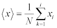
In most biomedical time series, they usually consist of property similar to the increments of random walks. To convert the noise signal into a random walk like time series, the data are subtracted by the overall mean value and then integrated along the time series.
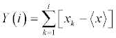
where i = 1, … , N; Y(i) is the random walk signal at frame i of time series; Xk is the original data signal; and is the overall mean value of time series, given by
After subtracting the angle data of cervical signal by its overall mean, and integrating along time series, a random walk like structure can be observed in Figure 4, as compared to the original signal in Figure 3.

Figure 4: Random walk like structure of the vertex M6 at cervical spine time series.
When comparing to the random walk structure to white noise, it is obvious that the plot of it (Figure 5) does not result in going up and down as observed from the plot above. The white noise is generated by random with variance of 0.01 and behave as Gaussian.

Figure 5: Random walk structure of white noise.
In the experimental time series, there are local fluctuations with both large and small magnitudes. The way to analyse this local structural variation is to divide the time series into segments and compute the local RMS corresponding to each segment. The process is to divide the time series into non-overlapping segments of equal size.

where Ns is the number of segment in a scale of s; N is the total number of frames; s is the length of equal-sized non-overlapping segment; and, int( ) is a function to get the floor value after the division. The experimental time series have a total of 5400 frames. For example, when the length of equal-sized non-overlapping segment is set to 600, it results in nine segments with nine local RMS values.
In biomedical time series, slow varying trends exist. Then, detrending the data is necessary in order to quantify the invariant structure in scale and reveal the variations around these trends. A polynomial fitting is applied to extract the trend of each segment. Linear, quadratic, cubic, or even higher order polynomials can be used in this fitting procedure. The local fluctuation can then be computed for the residual variation when compared to the fitting.
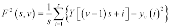
where F2(s, v) is the square of the RMS based on the local trend; s is the segment length; v is the segment 1, … , Ns ; Y [ (v - 1) s + i ] is the time series signal at particularly frame [ (v – 1) s + i ]; and yv is the fitting polynomial in segment v.
The application of detrending process on the experimental time series is to distinguish the local fluctuations of the spinal movement within each divided segment. The regression lines are the trend lines which represent the local tendency of spinal movement. Using the RMS computation, it measures how much the local fluctuations are different from the local tendency on the movement.
The time series have both the fast and slow changing fluctuation characteristics. The overall RMS is influenced by choice on the length of segment. Fast changing fluctuation is influenced by segment with shorter sample length, where slow changing fluctuation is influenced by segment with longer sample length. The scaling function of the overall RMS should then be computed for multiple segment sizes. It features both the fast and slow changing fluctuations that influence the structure of the time series.
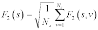
where F2(s) is the standard detrended fluctuation function at time scale s; s is the segment length; Ns is the number of segment in a scale of s; F2(s, v) is the square of the RMS based on the local trend; and v is the segment 1, … , Ns . In this case, the time scale is chosen with segment length [16, 32, 64, 128, 256, 512, 1024]. These segment lengths are chosen for the sake of the computation of log function later on. There are a total of seven scales that compose the overall scaling function.
Different segment lengths within the experimental time series represent how long the period of time is under investigation. Shorter the period reveals more the local fluctuation in spinal movement. Whereas the longer the period, it tries to compare the fluctuation to a relatively more stabilized posture. When the period is long, there is an averaging effect that averages out the large and small magnitudes of fluctuations, which eventually results in a stabilized posture.
The fitting polynomial is usually chosen with order between one and three [15]. Figure 6 illustrates the difference between the three orders. A high value of order might results in overfitting for time series. The RMS values are compared in Table 2. By comparing the RMS values and avoiding overfitting, first order polynomial fitting is chosen. DFA identifies the fractal structure as the power law relation among the RMS computed for multiple scales. The power law relation is represented by the slope of the regression line. Figure 7 illustrates the log-log plot of the local fluctuations and overall RMS versus multiple scales.
| Order | |||||||||
|---|---|---|---|---|---|---|---|---|---|
| 1 | 33.23 | 45.31 | 31.55 | 127.42 | 24.79 | 55.32 | 48.46 | 29.05 | 37.50 |
| 2 | 29.04 | 12.81 | 31.47 | 96.05 | 24.65 | 26.23 | 20.73 | 28.38 | 18.99 |
| 3 | 11.09 | 11.31 | 18.29 | 39.32 | 24.60 | 25.88 | 14.13 | 18.69 | 15.78 |
Table 2: RMS values of segments by various orders of polynomial fitting.

Figure 6: Computation of local fluctuations by various orders of polynomial fitting.

Figure 7: Power law relation among RMS for multiple scales.
Hurst exponent (H) is defined as the slope of the regression line. It indicates the fractal structure of time series in single dimension. The value of it measures the local fluctuation by how fast the overall RMS grows with increasing segment sample size. From Figure 8, the overall RMS is growing alongside with the increase in segment sample size. The growth is faster in the experimental time series when compared to the white noise.

Figure 8: Regression lines for different q-th order RMS.
According to the previous log-log fluctuation function plot versus time scale, the white noise has the Hurst exponent close to 0.5, which means the time series tends to be an independent or short-range dependent structure. The Hurst exponent has value of 1.2 in the experimental time series, which indicates a random walk like structure with apparent slow evolving fluctuations.
The overall RMS variation can be seen increasing when the segment scale increases. That comes to the definition of H. However, within a time series that consists of multifractal structure, local fluctuations exists in both extreme small and large magnitudes. Since this is not present as a structure of normal distribution, in the case of monofractal time series, second order statistical moment, for example, variance, cannot be used alone. Consequently, multiple order statistical moment should be considered. Thus, the q-th order RMS is applied in order to extract the various magnitudes of large and small fluctuations in the case of multifractal DFA.
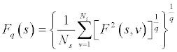
where Fq(s) is the q-th order fluctuation function at time scale s; s is the segment length; Ns is the number of segment in a scale of s; F2(s, v) is the square of the RMS based on the local trend; and v is the segment 1, … , Ns . With the q-th order varies from negative to positive q, it weights the influence of segment from small to large magnitude of fluctuations.
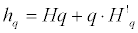
By the introduction of q-th order RMS, q-th order Hurst exponent can then be defined. It represents the slopes (Hq) of regression lines for each q-th order RMS. Figure 8 below illustrates the plot based on the experimental time series.
The q-order Hurst exponent Hq above is one of the several scaling exponents to reveal the multifractal structure of time series. There are other parameters derived from Hq to illustrate other aspects of the multifractal structure. The Hq is first converted to the q-order mass exponent, tq and is calculated by:
tq = q.Hq-1
In monofractal time series, the long range correlation is characterized by tq by linearly dependent q-th order with a single Hq.
Thereafter, the mass exponent (tq) is converted to the q-th order singularity exponent, hq by the equation:
where hq is the singularity strength and is the tangent slop of tq. The plot against q is illustrated as below.
The q-th order singularity dimension (Dq) is then defined by:
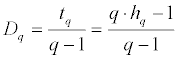
Dq is the generalized multifractal dimensions that are used together with tq in some research [2]. In both cases, they depend on q. When q = 0, D0 = -t0 = -1. The plot of Dq against q is illustrated as below.
When plotting the singularity dimension (Dq) against singularity exponent (hq), it reduces the multifractal spectrum into a small arc for the time series of monofractal and white noise. In the case of multifractal time series, it results a large arc where the difference between the maximum and minimum of hq are called the multifractal spectrum width, W. Figure 9

Figure 9: Multifractal spectrum as illustrated by Dq against hq.
The multifractal spectrum width (W) is about zero if the time series are monofractal or white noise. In the case of multifractal time series, W increases with the spectrum of multifractal structure.
The autocorrelation exponent (γ) can be estimated [10] from the equation below:
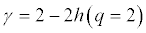
where h(q = 2) is the singularity exponent when q-th order equals to 2. For uncorrelated or short-range correlated data, h(2) is expected to have a value 0.5, while a value greater than 0.5 is expected for longrange correlations. Therefore, for uncorrelated data, γ has a value 1. The lower value, the more correlated is the data.
To ascertain the multifractality with the time series, it can be determined by analysing the randomly shuffled series from the same data set. The process of shuffling is to put the data into random order. The aim is to destroy all correlations. Then, the long-range correlations within the multifractal structure disappear and then become nonfractal scaling. On the other hand, the time series are said to origin based on probability density, if the Hq is about the same as before and after the shuffle. If multifractal structure is present in both original and shuffled time series, the multifractaility will show as a weaker one in the shuffled series.
After the shuffling process, the random walk plot goes from the scale of absolute maximum value about 2000 (Figure 5) down to about 150 (Figure 10).

Figure 10: Random walk plot of the shuffled time series.
In order to find out the multifractality of the time series, the original and shuffled time series are compared and analysed. The variation of the values of Hq vs q, tq vs q, hq vs q, and Dq vs q are illustrated in Figure 11-14. The y-axis are the values corresponding to various fractal parameters. The x-axis represents the change in the q-th order. The bolded lines shows the boundary between the minimum and maximum range of particular time series, that is, original and shuffled. This boundary is based on all trials obtained from experiment. The lines in between the boundaries are equally spaced showing the change of magnitude in range.
Figure 11: Plot of minimum to maximum range on Hq against q based on all trials of original (upper) and shuffled (lower) time series.

Figure 12: Plot of minimum to maximum range on Hq against q based on all trials of original (upper) and shuffled (lower) time series.

Figure 13: Plot of minimum to maximum range on hq against q based on all trials of original (upper) and shuffled (lower) time series.

Figure 14: Plot of minimum to maximum range on Dq against q based on all trials of original (lower) and shuffled (upper) time series.
It is obvious that the plot of original data is largely different from that of shuffled data. In the Hq plot, the shuffled data fall into the range of white noise while the original data represent the random walk structure. In the tq plot, it illustrates another variation between the original and shuffled time series. As the original time series exhibit multifractal structure, it results in a larger variation in tq values. In the hq plot, the shuffled time series shows a similar behaviour near the 0.5 value while compared to the original time series. In the Dq plot, it shows the difference in the variation on the dimension between the original and shuffled time series.
Further in Table 3, it shows the values of hqmin , hqmax, W and γ compared between the original and shuffled data. Values of γ of the shuffled data is quite close to 1, while that of the original data has a lower value. It is as expected since the correlations are destroyed in the shuffling process. This result demonstrates the fact that the multifractality in spinal curvature is predominantly due to long-range correlations.
| hqmin | hqmax | W | γ | |
|---|---|---|---|---|
| Original data | 0.90 ± 0.11 | 1.59 ± 0.10 | 0.69 ± 0.13 | 0.00 ± 0.20 |
| Shuffled data | 0.46 ± 0.04 | 0.55 ± 0.04 | 0.09 ± 0.05 | 1.01 ± 0.06 |
Table 3: Values of singularity exponent, multifractal width and autocorrelation coefficient between original and shuffled data.
One might think that the variations within a static posture are simply the representation of uncorrelated white noise added together on static and stationary series of data. It assumes that these large and small fluctuations are noise. Another possible explanation is that there exists finite range correlations in space. In other words, the current data are influenced by the near and most recent data. However, the fluctuations are random in a long run. Along a similar scope of thinking, the fluctuations in the spinal curvature consist of long-range correlations. In this case, the spinal curvature data at any instant are influenced by relatively remote intervals, and the influence would decay in a scale-free fashion.
The H illustrates the fractal structures with different characteristics between random walk like and noise like time series [15]. When H falls in the range between 0 and 1, the time series are said to have noise like structure. If it is above 1, the time series consist of a random walk like structure. When H is in the range between 0 and 0.5 or between 0.5 and 1, the time series are said to have long-range dependent structure. In the case of range between 0.5 and 1, the time series have correlated structure, whereas the range between 0 and 0.5 is said to have anticorrelated structure. In particular when H equals to about 0.5, the time series are said to have an independent or short-range dependent structure. The other particular cases to note are the Hurst exponent having values of 1.0 and 1.5, which correspond to a pink noise and Brown noise respectively. The pink noise separates between noises H < 1 that have more apparent fast evolving fluctuations, and random walks H > 1 that have more apparent slow evolving fluctuations.
It shows that there is dependency between the slopes Hq of the regression lines and the q-th order in the case of experimental time series. When compared the small and large segment sizes, there is difference between qRMS for positive and negative q-th order. Local fluctuation with either large or small magnitude can be distinguished by using small segment sizes. The scale on magnitude of local fluctuation can be revealed by positive and negative q-th values corresponding to large and small magnitude respectively. In the case of large segment sizes, they go across several large and small magnitude of fluctuations. Therefore, the local fluctuations are averaged out by each other, hence appears to have convergence with large segment sizes.
Within the experimental time series, the large and small magnitudes of fluctuations represent the large and small spinal movements along the time. From the perspective of motor control system in a static posture, the human body tries to stabilize itself in every moment. The spinal movement is said to be the responsive action initiating to balance the human body. Previous research has found that human body has different types of response systems which results in different response time. The reaction can be very quick on some types of responses, while some may need longer period of time. With regard to postural sway and generally for the whole body, there are four types of response pathway and results in different latency time, as shown in Table 4 and Figure 15 below [16].
| M1 response | 30 to 50 ms latency |
| M2 response | 50 to 80 ms latency |
| Triggered reaction | 80 to 120 ms latency |
| Reaction-time response (M3) | 120 to 180 ms latency |
Table 4: Four types of responses.

Figure 15: Plot on latency time based on various responses.
Given the various types of responses affecting the postural sway, hence the spinal movement, the large and small movements might then be said as the scale depends on how much the human body tends to stabilize itself. The Hurst exponent is then defining the correlation of movement with respect to various order and time distance. Through the conversion from mass exponent into singularity strength, it defines the width of the multifractal spectrum, while the singularity dimension defines the height of it. Altogether, the multifractal spectrum defines the variations on the correlated spinal movement on postural sway. From the previous physiological findings on various types of responses, the variations on the large and small fluctuations might then be the resultant movement accumulated from the various responses due to different time latencies. Further speaking, that reveals how unstable the human body is at that particular moment. Larger the movement would mean more unstable that particular instant is.
From the comparison of plots in Figure 11-14 and the statistical summary in Table 2, it is obvious that the plot of original data is largely different from that of shuffled data. As compared to the plots from previous section in illustrating the difference between the multifractal data and monfractal / noise, the figures show the similar differences in plots. It suggests the fact that the origin of multifractality is due to both probability distribution and long-range correlation. It illustrates that the original data correspond to the multifractal data, and the shuffled data correspond to the noise. However, long-range correlation is dominant as suggested by the large reduction in multifractal width. Values of γ of the shuffled data is close to 1, while that of the original data has a lower value. It is as expected since the correlations are destroyed in the shuffling process. This result demonstrates the fact that the multifractality in spinal curvature is predominantly due to long-range correlations.
At this moment, the experimental time series is said to have revealed the fractal structure and indicates that it contains multifractal dimensions. One can possibly said that there are multiple strategies utilized by the motor control in response to unstable human body posture.
Detrended fluctuation analysis was applied to analyse the postural sway time series obtained from positional skin surface data captured by retroreflective optical markers. The postural sway exhibits random walk characteristics in the analysis. Further analysis based on multifractal detrended fluctuation analysis was also applied. It reveals the multifractal properties that are found in healthy subjects. The degree of multifractuality gives a hint on the multiple strategies in motor control. It brings the human body into a stable static posture by counterbalancing the subtle unstable sway as a result of physiological features, e.g., inspiration, inside the body, along the time dimension. However, the correlation between the multifractal characteristics revealed and the multiple strategies in motor control has to be further validated with more data sets.