1D, 2D, 3D: 1-, 2-, 3-dimension of spatial mapping with respect to the coordinates x, y, and z; a: Constant of Archie equation; α, β, γ: Tripotential electrode configurations; B: Magnetic field induction; C: Current electrode; CAES: Compressed air/gas energy storage; d: Bulk density; dbr: Brine density; dg: Gas density; Δgx, Δgy, Δgz Residual component of gravity field with respect to the background; EMI: Electromagnetic induction; ERT: Electric resistivity tomography; FWI: Full waveform inversion; GHG: Greenhouse gases; gx, gy, gz Gravity field components; gzx, gzy, gzz Gradients of gz; L1, L2 Minimization method of robust blocky and least squares normalization, respectively; L-BFGS Limited-memory Broyden-Fletcher-Goldfarb- Shanno of the quasi-Newton technique; m: Cementation factor of Archie equation; n: Saturation exponent of Archie equation; Ω: Ohm, electrical resistance unit; p: Pressure; P: Potential electrode; Φ: Porosity; R: Gas constant = 287.058 J/(kgK); RMS: Root mean square; ρ: Electric resistivity; ρa: Apparent electric resistivity; Sg: Gas saturation; t: time; T: Temperature; TDS: Total dissolved solids; TEM: Transient electromagnetic induction; Tx, Rx: Transmitter and receiver coil of EMI method; Vp Velocity of primary seismic waves; Vs Velocity of secondary seismic waves

One unprecedented challenge facing the human being is the energy resources, and its coupling with global climate change and warming from greenhouse gases, GHG. The anthropogenic GHG stems from burning fossil fuels which has a finiteness supply. Mitigating GHG demands developments of viable alternative of renewable energy resources including hydroelectric, biomass, solar, wind, marine (wave/ tides) and geothermal sources. Most of these sources are vulnerable to the climate vagaries, i.e., intermittent, and need buffer storage, such as a compressed air/gas energy storage (CAES). The daily electricity demand is constantly changing while the surplus renewable generation is put into storage. The basic CAES approach is as follows: When electricity generation is greater than demand, the energy surplus is used to compress air in the storage. When generation is less than demand, pressurized air is withdrawn

from storage and used to drive electricity turbines. Advantages of renewable energy storage are (1) balancing power demand and intermittent renewable energy production, (2) bridging temporal mismatch (disparity) between renewable energy production (off-peaks) and demand (peaks), i.e., storing off-peak energy supply to use it during peak demand periods, and (3) offering large buffer capacity to meet any disruptions in energy supply. The underground geology offers an adequate option for short- and long-term storage (hourly to seasonally) of huge energy quantities such as CAES, e.g., [1,2]. The North German Basin delivers favorable conditions (geological, geochemical) for underground space utilization including CAES in porous media (e.g., depleted gas fields or saline aquifers) and salt caverns (natural and artificial). However, this large scale use of this geologic energy storage induces secondary effects in the geologic subsurface, including pressure increase, migration of reservoir fluids, geochemical and biological changes, and geo-mechanical stresses as well as possible leakage of injected fluids or gases into drinking water aquifers [3]. In geologic energy storages, the gas replaces the pore brine causing strong changes in elastic moduli, density and electric resistivity. These physical contrasts justify the application of integrative geophysical techniques for monitoring this geo-storage. Since some years ago Germany practices a turnaround in the energy policy (German “Energiewende”) and is currently leading in the production of solar and wind energy [4]. Germany decided to phase out nuclear energy generation until 2022, which further accelerates the switch to renewable energy sources. Wind energy is produced mainly at the coastal areas (on-shore and off-shore) of North Germany which is characterized by high wind velocities (Figure 1). We started 2012 an interdisciplinary joint research project ANGUS+ dealing with impacts of using geologic subsurface as a thermal, electric or material storage in context with alternative energy resources [3]. Using numerical simulations we show here some results of the feasibility study by applying geophysical techniques of elastic full waveform inversion (FWI), electric resistivity tomography (ERT), transient electromagnetic induction (TEM) and gravity. The goal is to explore the capability of these multi-techniques to map and monitor deep CAES reservoirs and potential CAES leakages in the shallow groundwater aquifer. At first we present briefly basics of the applied geophysical techniques then show and discuss examples of mapping and monitoring results from deep CAES reservoirs and a CAES leakage plume in shallow groundwater, and finally give a summary and conclusion.

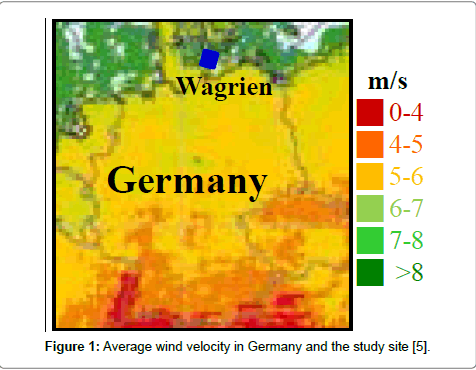
Figure 1: Average wind velocity in Germany and the study site [5].

Here we review briefly the geophysical methods of FWI, ERT, gravity and TEM applied in this numerical study.

Seismic Full Waveform Inversion (FWI)

Classical seismic travel time based tomographic approaches are limited in resolution to the first Fresnel zone. In the (spatial) FWI, the resolution can be significantly enhanced by incorporating phase and amplitude information of the whole recorded wave field (in addition to travel time information of specific waves) in the inversion process. The FWI aim is to minimize the data residuals δu = u^mod - u^obs between the modeled datau^mod and the field data u^obs to deduce high resolution models of the elastic material parameters in the underground. To solve this nonlinear optimization problem an appropriate objective function E has to be defined. Similar to Asnaashari et al. [5], the following objective function is used:

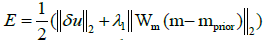(1)

Where the term denotes the L2-norm of the data misfit and a weighted L₂-norm of the difference between the model parameters m and prior model information mprior used for model regularization. The parameter λ₁ balances the contributions of the data misfit and the model regularization term, while the spatial variable weighting factor W_m defines the updated parts of the model during the inversion process. Like Asnaashari et al. [6], the magnitudes of the spatial weighting factors are based on elastic reverse-time migration results to spatially restrict model updates to the storage formation. The objective function Equation 1 can be minimized by iteratively updating the model parameters m_n (P-wave velocity V_p, S-wave velocity V_s, density d) at iteration step n, starting with an initial background model m₀, using the Newton method [7]:

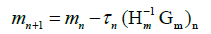(2)

with the gradient of the objective function Equation 1 with respect to the elastic model parameters

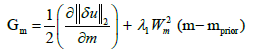(3)

and H_m as the second derivative of the objective function (Hessian). As the explicit calculation of the Hessian in the time-domain requires high computation time, the quasi-Newton L-BFGS (Limited-memory Broyden-Fletcher-Goldfarb-Shanno) technique is used [7,8], where the product of the inverse Hessian with the gradient G_m is iteratively approximated by finite differences.

The effective calculation of the time-domain gradient directions with the adjoint method for different model parameterizations are described in, e.g., [9,10]. The step length τ_n is estimated by a linesearch satisfying the Wolfe-conditions [7] to assure a fast and accurate convergence of the L-BFGS algorithm. To assure model smoothness, a weak wave number domain filter is applied to the estimated search directions at every iteration step. In time-lapse FWI, the data residuals are modified according to

δu=({u^mod(t₁) − u^mod(t₀)} − {u^obs(t₁) − u^obs(t₀)})(4)

where δu denotes the difference between the modeled and the field data at time steps t₀ (baseline model) and t₁ [11]. This redefinition of the data residuals leads to a stronger focusing of the model updates at reservoir level.

ERT technique

At first we introduce briefly the approach for optimized electrode configurations applied here for surface, borehole and combined surface-borehole surveys. For these surveys ERT data acquisition can be conducted in the tripotential 4-pole configurations α (CPPC, C = current electrode, P = potential electrode), β (CCPP) and γ (CPCP). For an N collinear multi-electrode array, a whole comprehensive data set consists of [(N-1) (N-2) (N-3)/8] independent non-reciprocal quadrupole configurations [12]. The effective comprehensive data set results from excluding the redundant configurations of less stable inversions from the whole set, i.e., γ configurations and those of very large geometric factors [13]. The resulting comprehensive data set is still huge, e.g., a pair of 32 borehole electrodes yield >106 data points. It can map subsurface targets with the highest possible resolution but at very long acquisition times, i.e., poor temporal resolution and high costs. Therefore, we apply here an optimization approach based on the model resolution matrix, e.g., [14,15]. It searches for electrode configurations that maximize the resolution of survey results [16]. We generated optimized data sets of practical sizes of up to 2% only of the comprehensive data set (i.e., ≤ 20,000 data points) but with almost the same spatial resolution. Comparative studies of diverse configurations (standard and non-standard) show the superiority of the optimized configuration results, e.g. [17]. Pore storage formations consist of a highly resistive matrix (e.g., sandstone) and conductive pore brine saturant. The bulk resistivity (p) resulting from the air/gas displacing the brine is predicted by Archie’s law [18]:

Where pbr is the brine/water resistivity, ϕ the porosity, S_g the gas saturation and a, m and n are Archie constants. The separate phases (matrix, brine and gas) are assumed without any interaction. The electrical conductivity of the storage formation is caused mainly by the electrolytes of its pore brine. In the North German Basin, temperature (T), pressure (p) and particularly the salinity or total dissolved solids (TDS) increase with depth. Increasing TDS and T causes a dramatic decrease in the resistivity, e.g., [19]; Schlumberger log interpretation charts, 2009. The TDS rise increases the number of ions carrying electrical currents. The T rise increases the salt solubility and decreases the brine viscosity which in turn enhances the ion mobility. The p increase, on the other hand, causes a slight increase in the resistivity due to the closure of cracks. However, this effect decreases with increasing depth and is negligible at pressure >0.3 GPa, e.g., [20]. In formations of the North German Basin, the average vertical gradient (with depth) approaches 100 mg/L/m for TDS of brine, 0.03°C/m for T and 22.6 kPa/m for p, e.g., [21]. In our numerical simulations, ERT surveys are conducted by placing electrode arrays at the surface and in boreholes. The storage targets host these vertical borehole arrays at an aspect ratio mostly of 1, i.e., array lengths are equal to their offset, to achieve a reasonable spatial resolution of the survey results. Sometimes the aspect ratio is increased (up to 2) to increase lateral coverage on the expenses of the resolution and vice versa [17]. The electric bulk resistivity models are parameterized by applying almost realistic values for the input parameters of Archie Equation 5 that are prevailing in the North German Basin. A 2.5D forward and inverse ERT modeling is carried out using modern codes (RES2DMOD, RES3DMODx64 and RES2DINVx64) based on algorithms by, e.g. Loke et al. [22]. The forward modeling code is applied to generate synthetic data sets using optimized electrode configurations for the different surveys. These data sets are generated after CAES injections in the storage reservoir. The data quality (0.6% average simulation error) is confirmed by results of tests on a homogeneous model with a constant p value. In the ERT inversions, diverse setup constraints (mainly regularizations) are applied. These include the minimization methods of least squares (L₂) or robust blocky normalization (L₁), and initial models of a constant homogeneous resistivity or an approximate inverse model, e.g., [23]. To minimize the ambiguity problems of non-uniqueness in the solution, ERT data are inverted with incorporating mapping data of the subsurface. For geostorage monitoring purposes this information may be well known from prior (baseline, seismic, logs) surveys, e.g., [24].

Gravity modeling method

Gravity studies are conducted here by 3D density modeling to test the technique capability for detecting and monitoring CAES plumes and their temporal variations in the underground (reservoirs and leakages). Rock densities depend on the mineral composition, porosity and its content (fluid and gas), p, T deformations etc. The injected CAES in saline reservoirs displaces pore brine and causes a drop of the bulk density which in turn causes a decrease in the gravity components and gradients. The bulk reservoir density (d) of partial gas saturations is given by [25]:

d=(1 − ϕ) + [d (1 − S_g) + d_g S_g](6)

where d_g, d_m and d_br are the gas, rock matrix and brine/water density, respectively, and S_gthe gas saturation. Dry air density is calculated as a function of depth (i.e., p and T) by:

d_g=p/(RT)(7)

Where R is the gas constant=287.058 J/(kgK) for dry air. Obviously dbr depends on the water density, TDS, p and T and is calculated as described in Batzle and Wang [26]. For calculating these densities, we consider almost realistic values for TDS, p and T as a function of depth within the North German Basin. The Stratigraphy and average bulk densities applied in the modeling study at CAES storage and leakage sites are based on borehole measurements and data base of Geotectonic Atlas of north-western Germany [27-29]. These almost realistic density values of rock formations show wide variations from 2050 kg/m³ for top Tertiary formations to 2710 kg/m³ for the bottom pre-Permian formations, e.g. [21]. We use here the software IGMAS+ (Interactive Gravity and Magnetic Application System) designed for 3D gravity, gravity gradient and magnetic modeling, e.g., [30,31]. The model is extrapolated outside the volume of interest in all directions (about twice the model length) to avoid any edge effects. We calculated the gravity field components (g_x, g_y and g_z) and gradients (g_zx, g_zy and g_zz) before and after CAES injection, respectively, as well as their difference (residual) anomalies (Δg_x, Δg_y and Δg_z). Here we show only the vertical component Δg_z maps calculated at the surface which reflect the strongest anomalies with respect to CAES reservoirs and leakages. We will discuss these gravity anomalies resulting from the CAES plumes and the least resolvable anomaly measurable by the modern microgravimeter with accuracy of 3-5 μGal.

TEM method

The transient electromagnetic induction (TEM) method can be applied on land, in the air and in the sea. Applying an electric current to a transmitter coil (Tx) and a rapid turn-off ramp (transient EM) induces a primary magnetic field with a strength depending mainly on the Tx-dipole moment and ground conductivity. This field generates Tx eddy currents within ground conductors which decays with time and in turn induces a secondary magnetic field (B). The temporal change in B (dB/dT) is measured as a decaying voltage by a receiver coil (Rx) at different time gates. This response curve can be transferred to the apparent resistivity (p_a) (dB/dT) directly proportional to used for a qualitative interpretation in a finite subsurface model. A conductive layer (e.g., saline aquifer) at shallow depths enhances response signals but decreases the penetration depth, and at greater depths enhances the penetration depth and TEM becomes insensitive to the underlying basement. Loops of high dipole moments and low frequencies are used to resolve the subsurface layers at great depths. Compared to surface ERT, TEM has advantages of surveying large areas without coupling problems to the ground, but limitations of the susceptibility to anthropogenic noises. Here we use the AarhusInv code for the forward generation of synthetic 1D TEM soundings resulting from a subsurface model of CAES leakage scenario and their inversions to recover this model [32]. Analogously to ERT, a hydro-geologic model resulting from multiphase flow modeling with the CAES plume are parameterized in a similar way (by using Archie Equation 5) to transfer them to resistivity models. This inversion relies on adaptive iterative fitting the calculated response of 1D models to the synthetic data. The code allows incorporations of constraints on the initial model (e.g., layer parameters) to minimize interpretation ambiguities.

Monitoring pore CAES reservoir

Here we present exemplary monitoring results of two growing CAES plumes injected in pores of thin brine reservoirs within the North German Basin. We introduce at first the synthetic site, and then the monitoring results of ERT and gravity techniques.

Synthetic pore CAES reservoir site

To approach more realistic modeling scenarios in this numerical study we selected the Wagrien site within the North German Basin to simulate pore CAES reservoirs (Figure 1). The site geology is reconstructed from data base of Geotectonic Atlas of Northwest Germany including seismic and borehole data [28,29]. This site has a model block of 29x28x5.5 km3. The subsurface consists of a thick succession of 14 sedimentary layers ranging in age from pre-Permian to Tertiary. Wagrien stratigraphy shows nearly horizontal layering with a gentle anticline fold (Figure 2). The succession includes two thin brine reservoirs of porous sandstone (5-30 m thickness), namely the shallow Rhaet formation (1-1.5 km depth) and the deep Quickborn formation (2-2.5 km depth). Both formations are potential pore reservoirs for CAES and are considered in this study. However, the stratigraphy shows an unconformity within the depth rang (0.7-1.0 km) of the shallow potential reservoir, where formations of the Lower Cretaceous, Lias and Rhaet disappear inside the anticline crest. The caprock for these storage formations consists mainly of siltstone, mudstone and salt layers which are nearly impervious representing seals for these potential CAES reservoirs. This CAES is injected in the top Rhaet/Keuper formation at three locations representing horizontal layering, anticline crest and anticline flank (Figure 2b, locations 1-3). In the deep Quickborn formation CAES is injected in the anticline crest (Figure 2b, location 4).

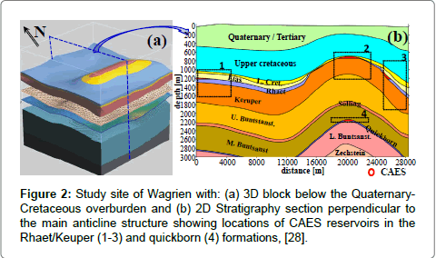
Figure 2: Study site of Wagrien with: (a) 3D block below the Quaternary- Cretaceous overburden and (b) 2D Stratigraphy section perpendicular to the main anticline structure showing locations of CAES reservoirs in the Rhaet/Keuper (1-3) and quickborn (4) formations, [28].

ERT monitoring results of pore CAES reservoir

Here we explore the capability of ERT technique to monitor the CAES plume in the Rhaet/Keuper layer below Wagrien site within the North German Basin (Figure 2b, locations 1-3). We consider here six different scenarios of varying geologic settings and injection times. The CAES is injected in a nearly horizontal layer, and at the crest and flank of the gentle anticline. These CAES plumes are observed at early, intermediate and late stages of injections. We may note that due to the disappearance of the Rhaet at the anticline crest (unconformity), the CAES plume is simulated in the underlying Keuper layer at this location. The geologic model is transferred into geoelectric model by applying the Archie Equation 5 with almost realistic parameterization, i.e. applying parameter values prevailing in this basin. In this equation we applied for the sandy reservoir 0.2 for ϕ, 0.08 Ωm (TDS about 100 g/l) for p_br, and 0.8 for S_g. The Archie constants a, m and n are substituted by values of 1, 2 and 2, respectively, which are commonly used in porous sandstone reservoirs [18]. Based on this petrophysical modeling, the CAES injection increases the bulk resistivity of the brine reservoir from 2 Ωm (without CAES) to 4-50 Ωm for saturations 30- 80% [17]. The ERT survey is conducted for this geoelectric model in a series of borehole electrode arrays within 600-1900 m depth range of the main storage targets (reservoir layer with overlying caprock and underlying aquitard). For these anomalous models caused by the injected CAES, synthetic data sets of apparent resistivity are generated using the code RES2DMOD and optimized electrode configurations for all applied CAES scenarios. These synthetic data sets are inverted using the code RES2DINVx64 with the a priori incorporation of the layer interfaces (without the unknown plume interfaces) to reproduce the initial subsurface model. For monitoring purposes, it is more likely to suppose that considerable subsurface information (including layer interfaces) is already available from previous (baseline) surveys such as seismic mapping and well logs. Our ERT data inversions reconstruct directly the true subsurface resistivity tomograms including the study CAES plume, i.e., no model differencing between tomograms with and without gas plume is necessary (unlike seismic). Figure 3 shows only the best-fitting tomograms of all differently independent inversions using different regularization parameters [17]. Every best-fitting tomogram shows least root mean square (RMS)-errors of <0.5% and iteration number almost of 5, and is optimized with the blocky L₁ norm for sharp interfaces. This L₁ norm yields significantly more accurate results (less RMS-error) than L₂norm. During inversion iterations, the applied L₁ norm allows the model resistivity to vary smoothly within each layer and abruptly across the layer boundaries. This is in accordance with our initial (input, true) subsurface resistivity model with abrupt changes at sharp target boundaries (cf., Loke et al. [33]). The low RMS-error value is explained by the good convergence of the synthetic data set toward the final solution. Obviously, our applied ERT technique reconstructs accurately the different single storage targets (the caprocks, aquitards and particularly CAES plumes) for all applied six scenarios. The technique is also capable to characterize these single scenarios from each other which is of an utmost importance for a successful monitoring strategy. The permanently installed (borehole) electrodes help to maximize the reliability of monitoring data. Modeled anomalies minimize the background effect and thus maximize the time-varying response caused here by CAES. A quantitative evaluation confirms the high resolution capability of applied ERT inversion codes as proven by its low values for the region of index and model residual relative to the input model [24]. Also adding random noise (1-5%) to the synthetic data increases the RMS-error values by a factor of 2-9 but slightly decreases the mapping capability of the techniques [16,34]. In conclusion our applied borehole ERT technique with optimized electrode configurations may be capable to monitor all these applied scenarios of thin CAES reservoir developments accurately if the inversion is geometrically constrained by a priori data on subsurface stratigraphy.

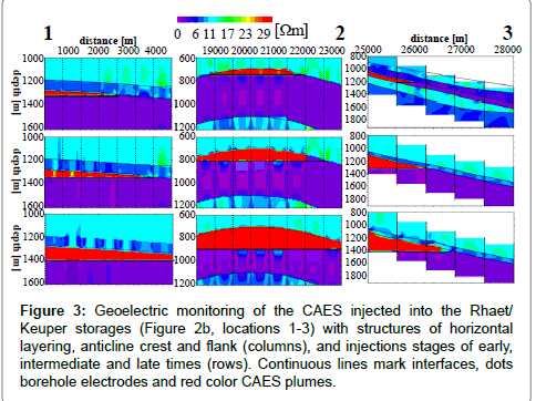
Figure 3: Geoelectric monitoring of the CAES injected into the Rhaet/ Keuper storages (Figure 2b, locations 1-3) with structures of horizontal layering, anticline crest and flank (columns), and injections stages of early, intermediate and late times (rows). Continuous lines mark interfaces, dots borehole electrodes and red color CAES plumes.

Gravity monitoring results of pore CAES reservoirs

Here we have simulated the growth of CAES plume with increasing injection time in the deep pore storage Quickborn under Wagrien site (Figure 2, location 4). The temporal development of the CAES plume is simulated by different successive time-lapses of increasing injection time, i.e., volume and depth to the plume bottom. Figure 4 (top) and Table 1 shows the depth to the base of the CAES plume and plume thickness at five different time-lapses. Usually the super light CAES propagates radially into the storage formation following the injection induced pressure gradient and accumulates mainly at the top of the anticline structure after the injection stop due to buoyancy effects [35, 36]. As mentioned before a realistic parameterization is considered for this location of the North German Basin. These subsurface scenario models are transferred to 3D density models by applying typical density values of the whole stratigaphy from literature [e.g., 25,28,29]. 3D density of CAES reservoir was calculated from Equation 6 by substituting ϕ by 0.15 and d_m by 2600 kg/m³, and calculating d_g from Equation 7. By applying the 3D gravity modeling program of IGMAS+, we calculated for these different time-lapses Δg_z anomalies relative to the background without CAES. Resulting maximum Δg_z amplitudes are listed for all time-lapses (Table 1) and only the measurable Δg_z anomalies (≥ 5 μGal, accuracy of micro-gravimeters) are shown in Figure 4, bottom. Results display the capability of the gravity method to monitor the temporal growth of CAES plume as clear negative anomalies starting from the size of time-lapse C and later. Time lapse C defines the least detectable plume scenario with 15 m thickness at this anticline crest. Early timelapses (Figure 4, A & Figure 4B) have Δg_z amplitudes below 5 μ Gal and thus cannot be detected with this technique. Results reflect the continuous increase of the amplitude and size of the mapped plume with increasing the injection time. Distinguishing the successive time-lapses from each other is hardly between C and D but clearly between D and E due to their corresponding maximum Δg_z differences of 2.9 and 10.2 μ Gal, respectively (Table 1). This good resolution is owed mainly to the large mass deficit resulting from our assumption of the full replacement of the pore reservoir brine by the CAES of 100% saturation and the absence of any temporal effects on the gravity. Obviously, time-lapse measurements do not require most corrections (e.g., free-air, elevation, Bouguer). However, some near surface changes (e.g., fluctuations of the water table) highly affect the gravity readings. Our gravity modeling on a water table at 10 m depth below the study site yields a measurable 5 μ Gal anomaly (microgravimeter accuracy) already for 0.5 m fluctuations only. Therefore, such fluctuations should be observed in wells to remove their effects from gravity readings.

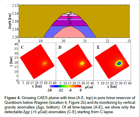
Figure 4: Growing CAES plume with time (A-E, top) in pore brine reservoir of Quickborn below Wagrien (location 4, Figure 2b) and its monitoring by vertical gravity anomalies (Δgz, bottom). Of all time-lapses (A-E), we show only the detectable Δgz (>5 μGal) anomalies (C-E) starting from C lapse.

CAES leakage in groundwater

Here we apply the different geophysical techniques to study CAES leakage in the near surface groundwater aquifer based on hydrogeological multiphase flow simulation. In the following we present at first the hydro-geological model, then results of potential field techniques (ERT, TEM and gravity) and finally FWI results.

Multiphase flow model

We have modeled a typical leakage scenario for CAES plume migrating upwards from a deep pore storage formation into a shallow fresh water aquifer within the North German Basin. In this multiphase/ multi component flow simulation we used TOUGH2-MP (EOS3) and PetraSim as graphical user interface for preprocessing to import the geological structure and post processing to analyze results [37]. Here CAES seeps for 10 years with 1 kg/s leakage rate into 500 m thick Quaternary aquifer consisting mainly of sandy sediments (Figure 5). Leaked CAES searches for release pathways along preferentially permeable zones (e.g., faults and buried channels). The upward CAES migration is driven by the lateral pressure in the underlying reservoir, buoyancy and density difference. In the aquifer CAES plume spreads with groundwater flow and accumulates below a surface cover of low permeable aquitard layer. The hydro-geological model after 10 years of the CAES leakage is used here for studying the applicability of the different geophysical methods to detect and map this leakage.

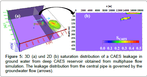
Figure 5: 3D (a) und 2D (b) saturation distribution of a CAES leakage in ground water from deep CAES reservoir obtained from multiphase flow simulation. The leakage distribution from the central pipe is governed by the groundwater flow (arrows).

Mapping CAES leakage by potential field methods

We present at first mapping results of ERT and TEM techniques, and finish with forward modeling results of gravity technique. The 2D CAES model simulated in the near surface of the North German Basin (Figure 5b) is transferred to resistivity model (Figure 6a) by applying the petrophysical Archie Equation 5. The same values of water and air saturations resulting from the hydro-geological modeling are considered here. We applied typical values for water mineralization or resistivity (average 25 Ωm) and ϕ-aquifer (0.20) prevailing at shallow groundwater aquifers of North Germany (e.g., [38]). ERT surveys are conducted using surface and borehole electrode arrays at 20 and 10 m intervals, respectively. Synthetic datasets using the optimized electrode configurations are generated for three survey designs conducted from the surface, in boreholes and from the combined surface-borehole. These data sets are inverted without any constraints and with incorporating information about the aquifer away from the unknown CAES leakage. Figure 6b-Figure 6e shows some examples of the resulting ERT inversion models. Reconstructed models show the capability of the ERT techniques (of different surveys and inversion constraints) to resolve the resistive anomalies of CAES leakage within the conductive aquifer. Obviously, the resolution of the inverted models is enhanced by: (1) applying the combined surface-borehole survey (compared to the single surface or borehole survey, cf., Figure 6b, Figure 6d, & Figure 6e), and (2) considering constrained inversions (compared to unconstrained inversions, cf., Figures 6b and 6c). Hagrey and Petersen [39] found that the mapping resolution of the near surface zone is enhanced strongly by adding borehole electrodes to the surface electrode array. This resolution enhancement (particularly with depth) is even superior to that resulting from applying the optimized electrode configuration instead of standard ones. We can see that the resolution of the surface survey decreases with increasing depth where the deep CAES anomaly show a smeared oversize and reduced amplitude. This is in accordance with the transverse equivalence for this type of a resistive anomaly inside the conductive medium of groundwater aquifer, where the technique is unable to resolve correctly the anomaly resistivity from its thickness (see below). Regarding TEM, this technique is applied on the same leakage model derived from the hydrogeologic CAES model of Figure 5b. Using the ERT input model (Figure 6a) three different 1D models were digitized representing the separate shallow and deep plumes of CAES leakages and their combination. Here AarhusInv code is used for forward modeling and inversion [32]. For these different models, 1D datasets (vertical electrical soundings) of apparent resistivity (response) curve were generated for ground- and air-based TEM surveys. These datasets are then inverted by posing constraints on the initial model (layer parameters). Prior knowledge on the model layers with the distribution of resistivity highs and lows may be guest from the qualitative interpretation of apparent resistivity curve obtained from the forward modeling. Figure 6f shows that the inverted (output) models reproduce their corresponding initial (input) models with a satisfactory misfit. This reflects the capability of TEM techniques (from ground and aero-surveys) to detect such shallow and deep resistive anomalies and to resolve them from each others. As anticipated the resolution decreases with depth, where the deep resistive anomaly shows more smearing effects (larger thickness and lower amplitude) compared to the shallow anomaly. Obviously, both ERT and TEM techniques are able to detect this resistive CAES leakage and to resolve its shallow and deep anomalies within the conductive groundwater aquifer. However, the resolution of these resistive air plumes in this conductive medium is governed by the equivalence principle of the transverse resistance (p_h=constant, h=layer thickness), where smearing effects increase the thickness on expenses of the resistivity amplitude, i.e., the amplitude is here underestimated (Figure 6). As we have shown applying the constrained inversion minimizes strongly this smearing effect and may help in recovering the true resistivity which in turn may yield more realistic CAES saturations by applying the petrophysical Equation Finally, the 3D gravity technique of forward modeling using IGMAS+ code is applied on 3D leakage model of Figure 6a, [30,31]. This leakage model is transformed to 3D density model using Equation 6. For the sandy aquifer we substituted ϕ by 0.20, d_m by 2600 kg/m³, d_g by 1.23 kg/m³and applied the same values for water and CAES saturations resulting from the multiphase simulation. Resulting Δg_z anomaly relative to the background (Figure 7) shows a high sensitivity to this shallow leakage in the groundwater aquifer. The anomaly amplitude depends strongly on the air saturation and leakage size. For this leakage, a negative anomaly approaches amplitude of up to 200 μGal which is far higher than the least measurable value of 5 μGal for microgravity. As mentioned before, this good resolution is owed mainly to the large mass deficit resulting from the replacement of the pore groundwater by the super light air and the assumed absence of any temporal effects on the gravity. Time-lapse data for monitoring purposes do not require most corrections but temporal shallow fluctuations of the water table highly affect the gravity readings. In conclusion, the applied 3D gravity technique shows high sensitivity to the mass deficit resulting from the leakage of the gas phase and its saturation changes, but the data should be corrected for temporal fluctuations of the groundwater table.

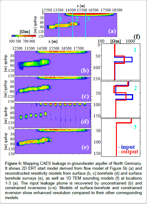
Figure 6: Mapping CAES leakage in groundwater aquifer of North Germany. It shows 2D ERT start model derived from flow model of Figure 5b (a) and reconstructed resistivity models from surface (b, c) borehole (d) and surface borehole surveys (e), as well as 1D TEM sounding models (f) at locations 1-3 (a). The input leakage plume is recovered by unconstrained (b) and constrained inversions (c-e). Models of surface-borehole and constrained inversion show enhanced resolution compared to their other corresponding models.

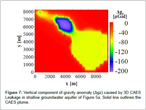
Figure 7: Vertical component of gravity anomaly (Δgz) caused by 3D CAES Leakage in shallow groundwater aquifer of Figure 5a. Solid line outlines the CAES plume.

Mapping CAES leakage by WFI

Based on the results of the multiphase flow simulation (Figure 5b) changes of the elastic material parameters due to variations of the gas saturation are calculated via an appropriate petrophysical relation. This is based on a Gassmann fluid substitution model [40] assuming a patchy gas-distribution [41], when the gas partially drains the fully water saturated aquifer. The resulting changes of the elastic material parameters are shown in Figure 8a- Figure 8c. A synthetic reflection seismic survey along the transect of 6 km length and 130 m depth is computed by solving the 2D isotropic elastic equations of motion with a time-domain finite-difference (FD) technique on a Cartesian grid [42,43]. The reflection seismic acquisition geometry consists of 500 vertical component geophones located at the surface. For the synthetic dataset 100 shots are recorded using a vertical impact source. The source signature is a 20 Hz Ricker wavelet. A free surface boundary condition is assumed on top of the model, while convolution perfectly matched layers [44] are used at all other boundaries. Due to the free surface boundary condition the data is dominated by the Rayleigh wave, which highly increases the nonlinearity of the inverse problem [45]. The synthetic seismic sections are the input data for the FWI. The initial model for the time-lapse waveform inversion at each time-step is the true elastic baseline model before the CAES leakage. No constraints to the time-lapse data, like sequential frequency/offset filtering or time windowing, are applied and all elastic model parameters are inverted simultaneously. The inversion results of the seismic data (Figure 8d- Figure 8e) are compared with the true changes of V_p, V_s and bulk density d_b (Figure 8a- Figure 8c). Due to the dominance of the Rayleigh wave in the time lapse data only V_s model variations could be recovered with some success, while the changes in V_p and d_bare underestimated. This is one of our preliminary results and further technique refinements are currently under investigation.

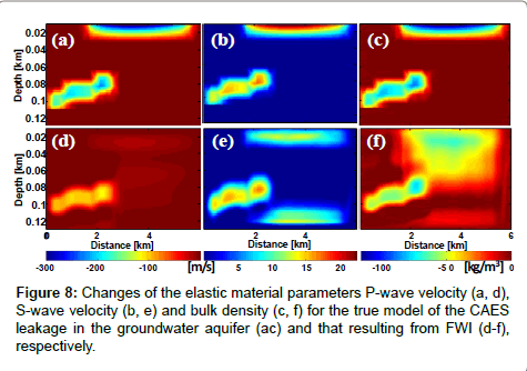
Figure 8: Changes of the elastic material parameters P-wave velocity (a, d), S-wave velocity (b, e) and bulk density (c, f) for the true model of the CAES leakage in the groundwater aquifer (ac) and that resulting from FWI (d-f), respectively.

Renewable energy resources are intermittent and need buffer storage to bridge time-gap between production and demand peaks. The North German Basin has favorable conditions (geology and geochemistry) and a very large capacity for CAES in saline formations. Geostorage of gas in porous formations causes strong changes in electro-elastic properties and density, and justify applications of multi-geophysical approach. These CAES targets are characterized by increased resistivity and impedance contrasts, and mass deficit. Using numerical simulations we study here the feasibility of the geophysical techniques of ERT, TEM, gravity and FWI in monitoring deep pore CAES reservoirs, and detecting their leakages in shallow groundwater aquifers below synthetic sites of North Germany. We generated synthetic data sets for different subsurface model scenarios of CAES reservoirs and leakages. Datasets are inverted using different constraints on the initial model. Results of this numerical study reflect the capability of our geophysical techniques to detect and monitor CAES plumes and leakages in the groundwater aquifer below the North German Basin. The constrained ERT inversions of optimized data sets acquired from surface, borehole and combined surface-borehole surveys can resolve well the slightly to highly resistive CAES plumes in the deep pore brine reservoir (extremely conductive) and the shallow groundwater aquifer (moderately conductive). Also the capability of ERT technique in resolving shallow leakages is highly enhanced for the combined surface-borehole survey compared to the separate surface and borehole surveys. The permanently installed (borehole) electrodes help to maximize the reliability of monitoring data by minimizing the background effect, i.e., maximizing the timevarying response caused here by CAES. Resistive CAES anomalies in shallow aquifers can be detected even by the TEM technique which is usually more sensitive to conductive anomaly. The applied gravity technique can detect pore CAES reservoirs in the deep underground, and can determine its lower boundary value of detectability, i.e., the least CAES quantity causing anomaly amplitude in the range of the accuracy of modern micro-gravimeters of 3-5 μ Gal. Moreover, the gravity method is sensitive to CAES leakages in shallow groundwater and the anomaly amplitude depends on the leakage size and CAES saturation. Also the FWI technique can map the shallow CAES leakage in groundwater aquifer by anomalies in the reconstructed Δ V_p, Δ V_s and Δd_b tomograms. However, these tomograms contain inversion artifacts and smearing effects related mainly to the dominance of the Rayleigh wave in the data. We may conclude that applied multi-geophysical techniques complement and confirm each other. CAES plumes cause strong impedance and mass deficits, and moderate resistivity highs, i.e., they are more sensitive for gravity and FWI methods. Applying the constrained inversion minimizes strongly the smearing effects and artifacts of inversions, and helps recovering the true electrical and elastic parameters which in turn may yield more realistic CAES saturations by applying adequate petrophysical equations. All results show that the resulting model resolution is highly enhanced by applying our concept of: (1) the multi-geophysical approach, (2) the optimized approach for surveys and data acquisitions, and (3) the constrained inversion with the a priori use of all available data. Currently we focus on refining the tomography technique of elastic FWI and the constrained inversions of all applied techniques. Our goal is to develop an integrative multi-geophysical approach for detecting mapping, monitoring and quantifying CAES and leakages at high resolution. For this purpose we conduct detailed sensitivity and resolution analyses for all these single techniques with respect to: (1) CAES dimensions and saturations, (2) adequate petrophysical approach (parameters and laws), (3) geologic and tectonic settings of storage sites, (4) post injection fracturing, (5) field setups and data acquisition techniques, and (6) various constrained inversion parameters.

Special thanks for E. Auken and A. Christiansen for providing AarhusInv program, and H.-J. Götze and S. Schmidt for providing the software IGMAS+. We thank D. Wehner, and B. Weise for computer work. This study has been carried out within the framework of ANGUS+ research project funded by the German Federal Ministry of Education and Research (BMBF).We thank project partners for efficient collaborations.