Drug Designing: Open Access
Open Access
ISSN: 2169-0138
ISSN: 2169-0138
Research Article - (2015) Volume 4, Issue 2
Finding the maximum tolerated dose (MTD) is the most important primary objective for Phase I oncology studies. The drug exposure and the toxicity event are the two components required for characterization of the MTD. Phase I trials currently require multiple subjects treated at numerous dose levels, with many of these subjects receiving doses of drug at less than predicted efficacious exposures. Further, these studies employ predefined, step-wise increments in doses that can result in inaccurate predictions of the MTD. Improvements to conventional adaptive dose finding designs to attain more accurate information on the extent of exposure and the time to event, with a more dynamic enrollment to facility better decision making are needed and have been the focus of previous published efforts. The EACRM dynamically extends the conventional adaptive dose finding designs by incorporating dose limiting toxicity (DLT) events as well as at-the-event information from each patient. An Accelerated Failure Time model with some tweaking to update the time to DLT for subjects who did not complete the entire DLT assessment period at particular time point was developed. Simulations, under a variety of assumptions, have indicated that the EACRM performed equal or better than the traditional 3+3 design in identifying the MTD and also outperformed the 3+3 design in other important operating characteristics such as the length of study, the number of subjects treated at above the MTD, and the total number of subjects.
<Keywords: Adaptive designs, Accelerated failure time model, Maximum tolerated dose,Dose limiting toxicity,Phase I
In Phase I oncology studies, the most important primary objective is to find the maximum tolerated dose (MTD). Drug exposure and toxicity events are the two major components required for characterization of the MTD. It has often been assumed in the literature as well as clinical practice, as a simplified approach, that the toxicity outcome can be observed before a given time T, and the assigned dose level would represent the drug exposure leading to the outcome of with or without toxicity before time T. Consequently, many Phase I oncology dose finding designs, including the traditional 3+3 fixed designs and various versions of adaptive continual reassessment methods (CRM) [1] have been operated under a set of distinct cohorts of patients with a predefined observational period (e.g. the first cycle) for tracking the toxicity outcomes. The dose escalation decision would be made periodically, requiring all the patients within the cohort of the assigned dose have been enrolled and followed up until crossing the finish line of the observational period.
In addition to the operational restrictions, strong clinical and statistical assumptions are made for those conventional dose escalation studies including fixed and adaptive designs: the observational period is chosen properly such that the intended toxicity incidence would follow the stochastic process according to the underlying population true incidence rate; moreover, the expected time of the onset for doserelated toxicity is assumed to be the same across different patients and all dose levels interrogated. While there might be situations where it would be possible to measure the two required components - drug exposure and toxicity outcome - with an approximation by fixing the observational period and using the assigned dose level, the strong clinical and statistical assumptions rarely truly hold. The duration for the observational period is often set up based on the assumed hematologic recovery period, more subjectively on the assumed toxicities that are expected, or based purely on practicality; otherwise, if a study stretches the observational period to capture delayed-onset toxicities, the dose-finding process will be substantially delayed before moving on to the next cohort. As a result, the conventional doseescalation designs that treat many patients at sub-therapeutic doses unnecessarily prolong the time of studies, are often inaccurate in determining true toxicity rates, and rarely allow estimation of clinical response at doses to be used in phase II studies. These designs also have the disadvantage of periodic closures and lengthy accrual time, and often lose momentum because of the episodic nature of accrual [2]. The operational and clinical challenges, along with major drawbacks including 1) the time to the toxicity event is not accounted for, 2) the extent of drug exposure leading to the onset of toxicity is not measured correctly, and 3) delayed-onset toxicities past the cut-off observation period are not captured, improvements should be made to attain more accurate information on the extent of exposure and the time to event, with a more dynamic enrollment to facilitate better decision making at the early phase, thereby increasing the probability of success in treating patients.
To address the major drawbacks as described above, statistical methodology has been proposed in the literature including using sequential designs for phase I clinical trials with late-onset toxicities (TITE-CRM) by Ying Kuen Cheung and Rick Chappell [3] via the maximum likelihood approach, and Bayesian approach by Suyu Liu and Jing Ning [4] for drug combination trials with delayed toxicities. The general pros and cons from either maximum likelihood vs. Bayesian approaches have been debated extensively in the statistical literature, and the debate is not the focus of this research. The objective of our research is to address the major drawbacks from the conventional designs by proposing a robust methodology that is readily implementable in real clinical practice. Furthermore, the operational hurdle of periodic closures is overcome by being able to enroll patients in a staggered fashion. The rest of this paper is organized as follows. We present our new methodology of determining the MTD along with the main algorithm in section 2 and conduct simulation studies to compare it with some existing methods in section 3. In section 4 we address our conclusion and raise some further discussion on our method.
Model specification
The proposed exposure-adjusted continual reassessment method (EACRM) assumes continuous enrollment of patients/subjects with a calculation of the estimated MTD for each subject enrolled at corresponding time point. An accelerated failure time (AFT) model with dose level as the covariate will be employed to characterize the time to dose-limiting toxicity (DLT). The proposed AFT model is:
where D is the dose level and T is the time to DLT. The AFT model assumes linear relationship between the mean of logarithm of time to DLT and dose level as α and β denote the intercept and slope, respectively. Moreover, σ is a positive parameter that controls the variability of the model and ? denotes the error term. In this paper we assume that T follows either a log-Normal or Weibull distribution. More specifically, under 1) log-Normal model,  and
and  under 2) Weibull model,
  and ? follows a standard extreme value distribution with density function
  .
.
As an incorporation of the time-to-event information, let δ be the indicator of DLT (δ=1 for DLT) and let w denote the weight of an observation. Essentially the weight factor will control the contribution to the likelihood function from each data point during the estimation process. Given a set of full data  and corresponding density function f, the problem can be well characterized under the framework of survival analysis and the likelihood function is written as

A frequentist approach based on maximum likelihood method with Newton-Raphson algorithm will be utilized for the model estimation process. To assign the dose level to the next subject entering our trial, predictions of time to DLT are made based on all m possible dose levels  with d0 mg starting dose and d mg increment.
where L is a prespecified toxicity assessment period of study and  indicates that we are predicting the 1/3 quantile of the time to DLT for the new dose level as it is the usual threshold for DLT rate allowed. Once the estimated parameters,
  ,
,  and
and  are obtained, we can update the estimation of time-dose curve given the formula derived as follows: for log-Normal model,
  ; for Weibull model,
  . Note that the estimates , and are different under two models.
Determination of the responses and weights
As introduced in section 1, the model we proposed is able to utilize not only the toxicity events but also the time-to-event information by specifying appropriate time responses  and weights
  in the AFT model. Although there is no unique mathematical approach for the weights, it is natural and practical to make some basic assumptions on them: 1) Given a specific time point during the trial, a non-DLT subject with longer survival period (e.g. 9 weeks without having a DLT) is expected to have a lower probability of occurring a DLT than one with shorter survival period (e.g. 2 weeks without having a DLT) and hence higher weight of surviving entire toxicity assessment period without occurring a DLT. 2) In general, the weight should be an increasing function of observed time t0 taking values in [0,1]. A weight of 1 indicates that the information from that individual is fully used in the model.
A good candidate for the weight is the conditional probability of completion, or no DLT given the observed time. For example, if the duration of the observation period is L weeks long and t0 is the observed time, then the conditional probability is given by P(T>L|T>t0). It will be generic if we want the weights to be independent of the distribution of T, since the true distribution may not be known in the real case. However, to calculate the weights, we have to assume a specific distribution. And we point out that a distribution with constant hazards will be sufficient when subject is on a particular dose level over the entire toxicity assessment period. Throughout this section we let T be the time to DLT with mean time to DLT λ and assume  with density function, which is a special case of Weibull distribution with shape parameter value of 1 given by
Note that this would assume constant hazard of observing DLT at each dose level. Under Bayesian framework, it is natural to consider a Gamma prior for λ, i.e., λ ∼ Gamma (a,b) with shape parameter a and rate parameter b. Then the corresponding density function is
It follows that the posterior distribution for λ remains to be a Gamma distribution: λ | t ∼ Gamma(a +1,b + t) . Meanwhile, recall that we allow at most 1/3 DLT rate when seeking the MTD, which gives us a restriction between λ and the duration of the observation period, L:
Then under an approximate relationship we have
Given all the information on distributions and parameters, now consider
If we fix λ =λ * then for 0 < t0 < L the probability of completing toxicity assessment period without DLT is

Moreover, it can be shown that T | t0 < T < L follows a truncated exponential distribution with density function
Therefore, the corresponding conditional expectation is
where  is the cumulative distribution function of Gamma (2,λ*).
Given the derivation of all the relevant probabilities and distributions as shown above, we determine the response and weight for each subject in the following Table 1.
| Progress of a Subject in Trial | Response(Ti) | Weight(wi) |
|---|---|---|
| Completed without DLT | L | 1 |
| Observed with DLT | tDLT | 1 |
| In Progress and t0+E(T|t0)≥ L | L | P*(t0) |
| In Progress and t0+E(T|t0)< L | t0+E(T|t0) | 1-P*(t0) |
Table 1: Specification of response and its weight in model.
Main algorithm for implementation
Based on the introduction to our model from above, at each time point that a new subject enters the trial, MTD will be re-estimated based on all available observations using a parametric survival regression model. Then a simple algorithm can be provided as follows assuming that at most n subjects are recruited for the study and the time of enrollment follows a certain distribution, e.g. an exponential distribution with rate τ:
1. First allow 3 subjects to go through the entire trial process with either completion or DLT as the outcomes and check certain futility criteria.
2. Starting from the fourth subject, proceed iteratively for 3≤ k ≤ n-1:
a. When the (k+1)-th subject enters the trial, determine the time on the toxicity assessment period, DLT status and corresponding weight for all k existing subjects: (T1,δ1,w1 ),…,(Tk,δk,wk).
b. Drop all non-DLT observations that have small exposures, e.g. less than 10% out of entire toxicity assessment period.
c. Perform survival regression based on the AFT model. Use effective data collected from above steps.
d. Obtain the 1/3 quantile predictions for time to DLT for all dose  and assign proper dose level Dk+1 to the (k +1) -th subject based on formula derived in section 2.1.
e. Determine if MTD is achieved based on clinically not significant change in predicted MTD and end the iteration if necessary.
3. Verify the estimated MTD and collect summary statistics for time and dose variables.
Note that the futility criteria and conditions for MTD attainment may vary by specific studies. However, some general guidelines are highly desirable. For instance, a negative sign of the estimated slope for dose is expected in each iteration and some convergence check for the dose assignment will be necessary when seeking the MTD.
Generalization of the weights
As an illustration of the mechanism of EACRM introduced in the previous sections, we first provide an application of the AFT model in predicting MTD with modified observations incorporating the weights specified above. This methodology was utilized in locally advanced rectal cancer study which administered investigational drug in combination with chemotherapy and radiation therapy. The toxicity assessment period was 8 weeks. The dose range planned to be investigated were 20–400 mg BID with anticipated MTD at 250 mg BID. For example, the next tolerable dose prediction was carried out using EACRM after enrolling 12 subjects. The data used and corresponding plot along with predicted tolerable dose using all available data are as follows (Table 2), (Figure 1):
| Subject Number | Dose Level | Time on Toxicity Assessment Period (weeks) | DLT Status | Weight |
| 1 2 3 4 5 6 7 8 9 10 11 12* |
20 20 20 20 30 60 70 70 70 80 100 110 |
8 8 8 8 8 8 8 8 1.9286 8 8 6.8571 |
No No No No No No No No Yes No No No |
1 1 1 1 1 1 1 1 1 1 1 0.9372 |
*Toxicity assessment period of 8 weeks was not completed by the time of subject 13 enters to the study. No DLT observed up to that point (6.8571 weeks) and so probability of not observing a DLT by 8 weeks is high (weight=0.9372).
Table 2: Example data from rectal cancer study.
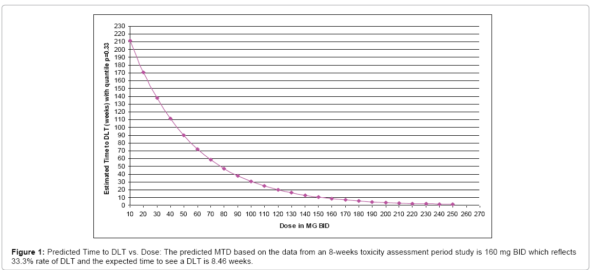
Figure 1: Predicted Time to DLT vs. Dose: The predicted MTD based on the data from an 8-weeks toxicity assessment period study is 160 mg BID which reflects 33.3% rate of DLT and the expected time to see a DLT is 8.46 weeks.
We note that our exposure adjusted design will handle the practical situation better in terms of the weights when fitting a model and provides a more reasonable prediction of MTD. Also, the prediction curve clearly indicates that the expected survival time E(T) decreases as the dose level D increases. But the previous designs assume no association between the expected time to DLT, E(T) and dose D since E (T)=E (1⁄ λ)= b/ (a-1). Therefore, a possible re-parameterization for λ is given by
 ,
,
which can allow such negative trend of the time-dose curve, where g(D) is a monotonically decreasing, positive function of dose D. Two simple but straightforward choices are 1) λ~~Gamma(aD,b) with  and 2) λ~~Gamma(a,b/D) with
  . These specifications are illustrated in the following two examples (Figure 2).
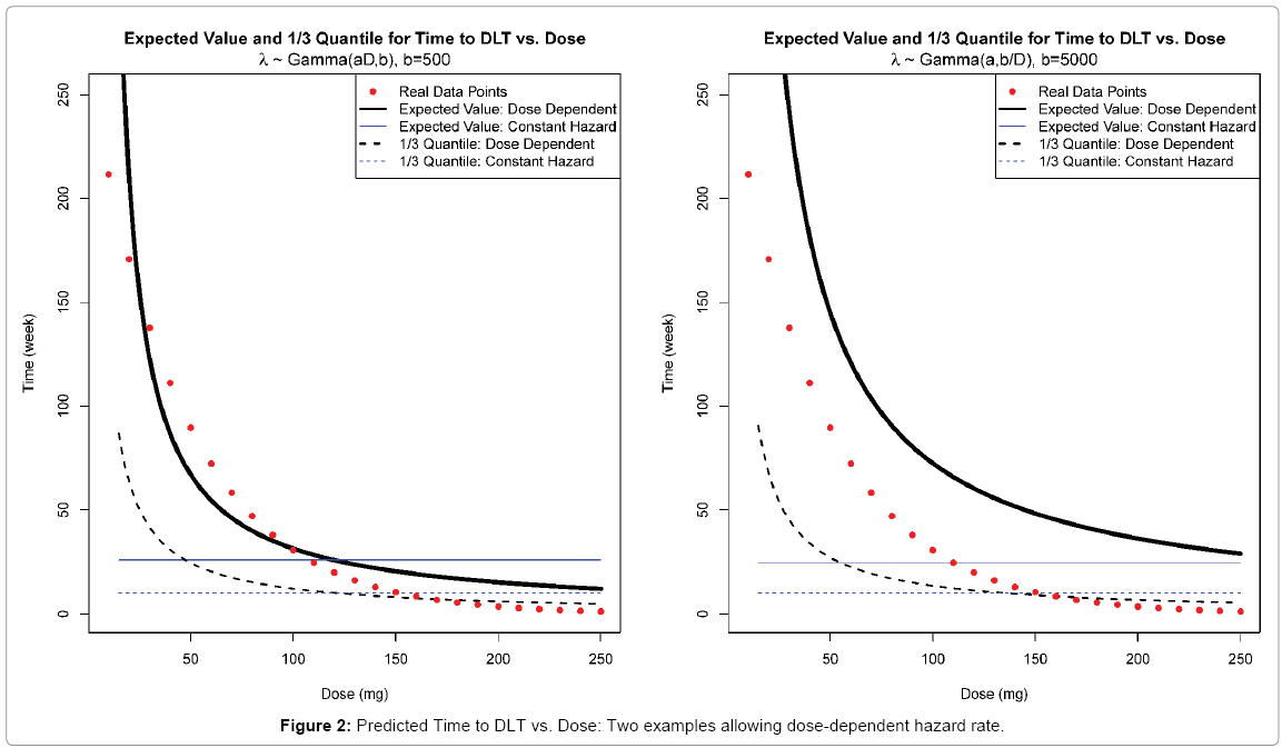
Figure 2: Predicted Time to DLT vs. Dose: Two examples allowing dose-dependent hazard rate.
The plots demonstrate reasonable fits to the real data with dose ranging from 10 to 250 mg. Hence we will consider both parameterizations of λ along with the original design that λ~~Gamma(a,b) as in section 2.2.
Note that due to the maximum of 1/3 DLT rate allowed, we anticipate similar restrictions on hyper-parameters a and b for both reparameterizations of λ as in section 2.2. However, since the dose level is involved, such restrictions can be only achieved at a given “targeted” dose level D0 , which leads to  . This relationship holds for both cases. Once D0 is specified which simply could be an assumed MTD, there will be only one free hyper-parameter, say, b. Then, as the rate parameter in Gamma distribution, b can be chosen as any positive constant. However, recall that
  for the first case and
  for the second one. To ensure that E (T ) > 0 for all possible dose levels starting from some initial dose d0 , we need
  for the first case and
  for the second. Therefore, generally the minimum value for b in the latter case is d0 times the one in the former case.
In this section, we run the simulations to study the performance of proposed EACRM design described in section 3 above. Depending on different assumptions on the true distribution of the time to DLT and the time-dose structure (in terms of parameterizations of λ), we consider the following 6 cases (Table 3):
| Prior Distribution used for Weight Derivation | Distribution for Time to DLT is Log-Normal | Distribution for Time to DLT is Weibull |
|---|---|---|
| Gamma (aD,b) | LN1 | W1 |
| Gamma (aD,b) | LN2 | W2 |
| Gamma (a,b/D) | LN3 | W3 |
Table 3: Parameterization and distribution matrix.
We compare our 6 cases with traditional 3+3 design and EACRM setting without using weights. For each case we run 1000 simulations based on two targeted MTD: 120 mg and 70 mg. The investigated dose range is 10-250 mg and toxicity assessment period is set to be 10 weeks. The maximum number of enrolled subjects is 40 for each trial (simulation). The arbitrary enrollment rate τ = 1/ 4 which leads to an average of 4 weeks waiting time between two consecutive subjects. We also assume the rate parameter for Gamma, b = 500 for LN1, LN2, W1, W2 and b = 3000 for LN3 and W3 to guarantee the probability of observing DLT within toxicity assessment period is not greater than 1/3 and E (T ) > 0 . If greater than 33% DLTs observed at first dose level tested then study is stopped for futility. The iteration of algorithm is stopped if change in predicted MTD is not clinically significant, i.e. less than 10% increment from current dose level.
Specification of true distribution
The parameters of true distributions that we choose are shown in the following Table 4.
Log-Normal Distribution:  |
||
| Parameter \ Targeted Dose | 120 mg | 70 mg |
| αLN | 2.6615 | 2.5500 |
| βLN | -0.0022 | -0.0022 |
| σLN | 0.2239 | 0.2239 |
Weibull Distribution:  |
||
| Parameter \ Targeted Dose | 120 mg | 70 mg |
| αW | 2.7820 | 2.8052 |
| βW | -0.0022 | -0.0022 |
| σW | 0.2379 | 0.3857 |
Table 4: Specification of true distribution.
The parameters are specified in a way that 1) they result in corresponding targeted MTD; 2) the slope coefficients of dose remain the same and 3) all the other parameters are comparable under different targeted doses and distributions.
Pseudo-Data: A guarantee for convergence of survival regression
During the early stage of simulation as subjects start to enter into a trial, the sample size may be small (e.g. 3 to 5), which usually results in a failure in convergence of the estimation under survival regression. Hence it is necessary to add a small number of pseudo-data into the regression as early observations. These pseudo data will be fixed throughout the study and will help in the model fitting process by solving convergence issues encountered during the early stage of the study. Appropriate weights will be assigned to them to reflect only a small degree of certainty. The pseudo-data we used are (Table 5):
| Observation # \ Variable | Time (weeks) | DLT Status (1 = Yes) | Dose (mg) | Weight |
| 1 | 10 | 0 | 60 | 0.09 |
| 2 | 8 | 1 | 60 | 0.01 |
| 3 | 10 | 0 | 120 | 0.07 |
| 4 | 8 | 1 | 120 | 0.03 |
| 5 | 10 | 0 | 200 | 0.04 |
| 6 | 8 | 1 | 200 | 0.06 |
Table 5: Pseudo-data Assignment.
Some general guidelines for pseudo data selection can be described as follows:
1. Consider 3 dose levels in lower, middle, and upper spectrum of the dose range to be investigated.
2. At each selected dose level in step 1 consider 2 data points, one with DLT occurring close to the end of toxicity assessment period and the other without DLT at the end of toxicity assessment period.
3. Assign very small weight (≤ 0.1) to those 6 data points. Also, consider the possibility of occurring a DLT event at selected dose level based on prior assumptions. For example, possibility of a DLT event at lower dose level is less compares to possibility of a DLT event at higher dose level.
A sensitivity analyses was carried out by altering the pseudo-data points generated using above guidelines. We point out that the pseudodata will not have notable impact to the final simulation results. In real practice, it is also very unlikely that the MTD will be achieved based on only a few data points with high degree of randomness.
Simulation results
We provide the summary statistics for all 6 cases for EACRM (LN1-LN3, W1-W3), 2 cases for EACRM without weights (LN0 and W0) as well as the 3+3 design (3+3) under both 120mg and 70 mg targeted doses. The results are listed in the tables below. The 25%, 50% and 75% label denotes the corresponding quartiles of the distribution of variables including the median (Tables 6 and 7).
| Case \ Stats. | MTD (mg) | Trial Size | Trial Duration (wks) | Med. DLT % | ||||||
| 25% | 50% | 75% | 25% | 50% | 75% | 25% | 50% | 75% | ||
| LN1 | 90 | 110 | 130 | 20 | 23 | 28 | 82.3 | 96.9 | 114.1 | 26.7 |
| W1 | 80 | 110 | 140 | 19 | 24 | 29 | 82.3 | 99.7 | 118.2 | 29.2 |
| LN2 | 90 | 110 | 130 | 19 | 23 | 28 | 81.7 | 96.0 | 115.4 | 26.7 |
| W2 | 80 | 110 | 140 | 20 | 24 | 29 | 82.8 | 100.4 | 118.8 | 28.6 |
| LN3 | 90 | 110 | 130 | 19 | 23 | 28 | 80.6 | 97.2 | 115.4 | 26.7 |
| W3 | 80 | 110 | 132.5 | 19 | 23 | 28 | 80.7 | 97.6 | 116.3 | 27.3 |
| LN0 | 80 | 100 | 120 | 21 | 24 | 28 | 87.8 | 102.4 | 118.3 | 21.7 |
| W0 | 70 | 100 | 120 | 20 | 24 | 28 | 81.5 | 99.7 | 120.0 | 24 |
| 3+3 | 40 | 90 | 120 | 15 | 24 | 30 | 90.0 | 144.0 | 180.0 | 21.4 |
Table 6: Summary Statistics for simulations under targeted dose 120 mg.
| Case \ Stats. | MTD (mg) | Trial Size | Trial Duration (wks) | Med. DLT % | ||||||
| 25% | 50% | 75% | 25% | 50% | 75% | 25% | 50% | 75% | ||
| LN1 | 40 | 60 | 80 | 16 | 20 | 25 | 67.6 | 85.2 | 104.8 | 33.3 |
| W1 | 10 | 50 | 100 | 14 | 19 | 24 | 58.0 | 80.9 | 105.4 | 33.3 |
| LN2 | 40 | 60 | 80 | 16 | 20 | 24 | 69.4 | 85.6 | 107.5 | 33.3 |
| W2 | 10 | 50 | 100 | 15 | 19 | 24 | 62.3 | 83.8 | 106.2 | 33.3 |
| LN3 | 40 | 60 | 80 | 16 | 20 | 24 | 67.6 | 85.4 | 103.6 | 32.1 |
| W3 | 10 | 50 | 90 | 14 | 19 | 24 | 61.5 | 81.1 | 104.4 | 33.3 |
| LN0 | 30 | 60 | 80 | 18 | 22 | 26 | 71.3 | 93.3 | 114.1 | 28.6 |
| W0 | 10 | 20 | 80 | 11 | 19 | 26 | 50.3 | 79.4 | 108.2 | 31.8 |
| 3+3 | 20 | 40 | 50 | 9 | 12 | 21 | 54.0 | 72.0 | 126.0 | 25.8 |
Table 7: Summary Statistics for simulations under targeted dose 70 mg.
Figures 3 and 4 provided below summarize and visualize the simulation process of 6 cases for EACRM under 120 mg and 70 mg targeted MTD. In each plot, we show the true dose-toxicity curve as well as the distribution of particular dose selected as MTD over 1000 simulations.
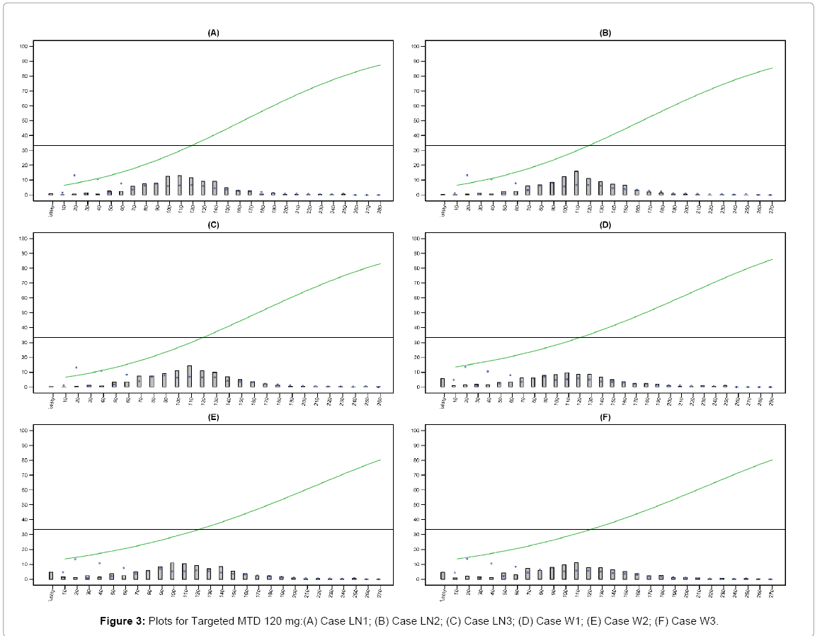
Figure 3: Plots for Targeted MTD 120 mg:(A) Case LN1; (B) Case LN2; (C) Case LN3; (D) Case W1; (E) Case W2; (F) Case W3.
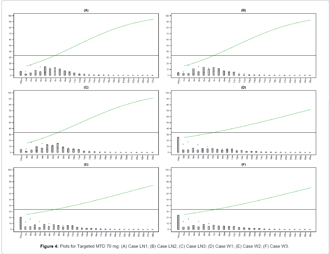
Figure 4: Plots for Targeted MTD 70 mg: (A) Case LN1; (B) Case LN2; (C) Case LN3; (D) Case W1; (E) Case W2; (F) Case W3.
From the simulation results presented in section 3.3 above, we claim some clear advantages of our proposed EACRM over the traditional 3+3 or standard survival regression model. First, by utilizing the DLT information as well as time on the study, the EACRM gives more accurate estimate of MTD than the 3+3 in general. Such improvement of accuracy becomes more significant as the targeted (true) MTD increases as the distribution of predicted MTD becomes more concentrated in terms of the variance and quantiles. It also allows for a more dynamic enrollment of subjects, facilitates better decision making thus requires shorter duration and potentially less subjects for a study. Meanwhile, the AFT model with weights depending on dose levels provides both high flexibility and efficiency in modeling, and the combination of frequentist approach for model estimation and Bayesian approach for weight determination shows more reasonable predictions for MTD.
When comparing the results from different distributions, we find that Weibull distribution demonstrates more variability when determining the MTD than the log-Normal distribution although it may require shorter duration of study. The EACRM keeps underestimating the true MTD slightly due to its conservative nature.
Although EACRM provided a satisfactory performance in terms of dose finding, it is commonly agreed among clinicians and biostatisticians that, as an adaptive design, the continual reassessment methods offer more aggressive dose escalation which may raise notable safety concern. Therefore, certain appropriate stopping criteria may be applied when selecting the MTD. Moreover, to handle a method with such a high flexibility in modeling, a good knowledge of both clinical trial and statistics will be essential. In practice, for first-in-human (FIH) studies that employ the EACRM, we have identified specific measures to ensure subject safety: 1) the first subject enrolled should complete the entire observation period prior to any dose escalations, 2) at the time of a DLT, any subject that enrolled at higher dose levels should have the option to reduce the current dose dependent on the toxicity observed, 3) some staggering of subject enrollment is required, thus we have required that in the event of very aggressive enrollment that no more than 6 subjects can be enrolled at the same dose level.
We also want to point out that there is always room for improvement regarding our proposed models and methods. For instance, a straightforward generalization of the time-dose relationship can be made by developing more complicated but flexible priors on λ when deriving the weights such as λ∼ Gamma(a0+a1D,b) or  . By introducing the intercept term we obtain a full linear function of dose level D which is able to fit a variety of decreasing curves which may be necessary since the pattern of time-dose curves can be more moderate as predicted MTD goes up. Another generalization is applicable on the distribution of T. When specifying the weights we consider an exponential distribution T~ Exp (λ) resulting in a constant hazard, which can be extended to a Weibull distribution, T~W (K, λ) with more general hazard given the shape parameter K and rate parameter λ. Then to obtain an appropriate posterior distribution, one may assume less informative Gamma priors for K and λ or even non-informative priors like π (θ ) ∝1 or π (θ ) ∝1 /θ , where θ is any parameter of interest. However, the corresponding posterior distributions have no known closed forms. Thus some sampling techniques for Bayesian inference such as Markov Chain Monte Carlo (MCMC) method may be needed for obtaining the posteriors and will be based on conditional distributions.
“AbbVie contributed to the research, and interpretation of data, writing, reviewing, and approving the publication. All authors are AbbVie employees and may hold AbbVie stocks or options.”