Fisheries and Aquaculture Journal
Open Access
ISSN: 2150-3508
ISSN: 2150-3508
Research Article - (2014) Volume 5, Issue 1
Mathematical models for the infection of juvenile Chinook salmon (Oncorhynchus tshawytscha) with Ceratomyxa shasta (a myxozoan parasite) in the Klamath River, California, were developed and parameterized with existing data. These models were then used to investigate the effect of three of the environmental conditions thought to be important to the parasite-induced mortality of juvenile Chinook salmon: the stream discharge during the exposure to parasite, the water temperature after infection, and the duration of the exposure to the parasites. The results of this study show that the sensitivity of parasite-induced fish mortality to environmental conditions is higher in spring than fall. Furthermore, the rate of parasite-induced mortality in fish increases with temperature within its range in the spring and summer, when a large number of juvenile fish migrate through the zone where the parasites are
prevalent. These results suggest that temperature may strongly affect the parasite-induced mortality of salmon in this stream. Observed seasonal difference in actinospore concentration could not be explained by the dilution effect due to changes in the stream discharge. This suggests the potential importance of other processes such as seasonal fluctuations in the release and natural mortality rates of actinospores. Finally, a sensitivity analysis was used to compare the effects of various environmental conditions. Under the conditions experienced in June 2008, increasing the discharge by 1 m3/sec would have an effect equivalent to decreasing the exposure duration by 0.26 hours or decreasing the temperature by 0.053°C. This type of analysis is expected to facilitate efforts to restore or mitigate salmon habitats.
Pacific salmon frequently suffer from infectious diseases. For example, the mortality rate of Chinook salmon (Oncorhynchus tshawytscha) is known to be increased by infection from bacteria [1-5], viruses [5,6], and metazoan parasites, [2,4,7-12]. However, understanding the relationship between parasite infection and associated mortality is complicated because the infection and subsequent mortality of fish are affected by environmental factors [13-17].
Ceratomyxa shasta is a myxozoan parasite and known to cause mortality of juvenile Chinook salmon. Recently, an elevated density of C. Shasta has been reported in a section of the Klamath River, California [18-21]. Juvenile Chinook salmon passing through the section, which is herein called the “infectious zone” have shown very high mortality rates in some years (62% in 2005 [18]). The infectious zone extends approximately from the Shasta River confluence (284 River km) to just below the Scott River confluence (229 River km). Because of the commercial, cultural, and other importance of this fish stock, the infection of juvenile salmon with C. Shasta has been studied intensively in the field and laboratory. The infection rate is currently thought to be affected by discharge [17], water velocity, and the density of C. Shasta in the water [15]. In addition, the rate of death of fish after infection appears to increase with temperature [14]. As these environmental factors are likely to be affected by the planned removal of dams [22], their relationship with parasite-induced salmon mortality needs to be elucidated for the Klamath River system.
The life cycle of C. Shasta requires two obligate hosts. The first is the polychaete Manayunkia speciosa from which actinospores of the parasite are released into the water. The infectious zone has a much greater density of infected polychaetes compared to other locations within the river [20,23]. The released actinospores infect juvenile Chinook salmon. After the infection, the actinospores may propagate within infected salmon and eventually kill the juvenile salmon [14,15]; however, the death of juvenile salmon is often delayed relative to the time of infection [15], complicating field measurements of parasiteinduced mortality.
The main objective of this study was to understand how the parasite-induced mortality rate of juvenile Chinook salmon in the Klamath River is affected by the prevalence of the parasite, the stream discharge, and the temperature. This was achieved by building models and parameterizing them with existing data. The primary sources of information were field and laboratory experiments conducted by Ray et al. [14,15]. They caged juvenile salmon in situ in the infectious zone for a defined period and then maintained the fish in the laboratory to investigate parasite-induced mortality [15]. In a second set of experiments, they varied the duration of field caging, and altered the laboratory water temperature to investigate the effect of temperature on the post-infection development of actinospores. Finally, they measured the in situ actinospore density and water discharge to determine the amount of exposure to parasites in the field [14].
Here, three models were developed to examine the infection process: a model for the stochastic infection of salmon with actinospores; a deterministic model for approximating the infection process; and a model representing the concentration of actinospores in the water. These models were parameterized with the data from Ray et al. [14,15] and existing stream-discharge information obtained from the USGS National Water Information System (http://waterdata.usgs.gov).
Stochastic infection process
Actinospores encounter and infect juvenile Chinook salmon, which die from the infection with some probability. Here, infection is considered “successful” if it can eventually lead to death from the infection; otherwise, it is considered “unsuccessful.” Therefore, infection is considered successful based on its potential to kill rather than whether it actually killed its host or not. Because parasite-induced death is delayed, an individual salmon can experience multiple successful infections in addition to multiple unsuccessful infections.
In this analysis, both successful and unsuccessful infections were assumed to be stochastic and independent of each other; all actinospores were assumed to be identical in terms of the infection process; and infection was assumed not to influence subsequent infections. Under these assumptions (independent, homogeneous, and memoryless), the number of individual-specific successful infections χ has the Poisson distribution, see [24]:
χ~ Poiss(μ) (1)
Where μ is the mean rate of successful infection. This is used for estimating the parameter.
Deterministic model: Approximation of the infection process
To model the dynamics of juvenile salmon abundance, a system of differential equations was developed, as follows:
 (2)
(2)
 (3)
(3)
Where S is the density of susceptible salmon without successful infection; I is the density of salmon successfully infected by C. Shasta; α is the infection rate; c is the concentration of actinospores; d is the instantaneous per-capita mortality of salmon from causes other than infection during the exposure period; and t is the duration of exposure. Ray et al. [15] used control groups to estimate the non-disease related mortality rate, and found that d was 0 during their exposure and laboratory-holding period. This largely reflected the lack of predators both in situ and in the laboratory and the use of antibiotics in the laboratory.
The density of susceptible salmon after exposure for time t is given by solving equation (2) after setting d=0:
S=So e-αct (4)
Where S0 is the initial density of susceptible salmon. Finally, the proportion of fish that eventually die from infection (m) is given by:
m=1-e-act=1-e-αE (4)
where E is exposure (calculated as the product of the actinospore concentration c and the exposure duration t). The unit for parameter E is the number of actinospores per liter of water. Consequently, the unit for the infection rate α, which also includes the filtration of water by fish, is the number of dead fish per liter of water filtered per unit time. Because the filtration rate of water is unknown in this study, it is included in the unknown parameter α to be estimated rather than estimating it separately.
Model for the concentration of actinospores in the water
The concentration of actinospores in the water was determined by their release from polychaetes, their reduction due to the infection of salmon, and their natural mortality, as:
 (6)
(6)
Where κ is the instantaneous release rate of actinospores from polychaetes, γ is the infection rate (including both successful and unsuccessful infections), N is the total density of salmon (N=S+I), and δ is the instantaneous per capita mortality rate of actinospores in the water. For a given environmental condition, therefore γ∝α. The difference between γ and α exists because not all infected salmon die after parasite infection. Therefore, γ>α. The uptake of actinospores by other organisms was assumed to be included in the natural mortality term δ , and was expected to be small due to the host specificity of C. Shasta.
The effect of the stream discharge (V:m3/sec) on the actinospore concentration (c) was incorporated. Assuming that the polychaete density and actinospore release rate per polychaete remain constant, κ can be expressed as:
 (7)
(7)
In other words, a high water discharge dilutes the concentration of actinospores in the water.
Because the processes governing the dynamics of actinospores are expected to be much faster than those governing salmon density, such that  , the expression for the actinospore concentration c is obtained as the following:
 (8)
(8)
where the star indicates that the concentration is at equilibrium. Therefore, if infection rate γand the per capita instantaneous mortality rate of actinospores (δ) is not affected by the discharge, the concentration is inversely proportional to the discharge, and may be written as:
 (9)
(9)
It should be noted that the assumption  implies that salmon and actinospores in the water equilibrate quickly in the time scale of the model, but it does not imply that the equilibrium concentration c* is constant in a longer time-scale. For example, c* can change because of slower changes in release rate κ and salmon density N. Parameter κ is discussed further in Discussion.
Sensitivity of mortality rate
In general, a sensitivity of mortality rate m with respect to any arbitrary parameter X is given by  . Thus, the sensitivities of the mortality rate to the duration of exposure t, the discharge V, or the temperature h were obtained by taking the derivative of the mortality function (5) with respect to the corresponding parameter. The sensitivity of the mortality rate to the duration of exposure is:
 (10)
(10)
the sensitivity of the mortality to the discharge is:
 (11)
(11)
and the sensitivity of the mortality to the temperature is:
 (12)
(12)
Where,  is given by the slope of the function relating α and h.
Parameters for the sensitivity analysis were estimated as outlined in the following section. For the actinospore concentration c, the average number of actinospores per hour per liter in June and September 2008 were calculated from the values in Ray et al. [15]. For the sensitivity calculations, the temperature h was assumed to be 18°C, and the duration of exposure t was assumed to be 24 hours. Furthermore, average discharge over a month was obtained from the USGS National Water Information System for June and September 2008 was used for V.
Parameter estimation and data
The two basic parameters to be estimated were the infection rate (α) and the actinospore concentration in the water (c). Infection rate can be a function of temperature, while the concentration can be a function of the stream discharge. These parameters were estimated from the results in Ray et al. [14,15] and existing stream discharge data.
Pr(χ>0)=1-e-μ
By letting, μ =αE probability (13) can be approximated by the deterministic model (5). In other words, by taking the mean probability over a large number of fish, this probability was interpreted as the finite mortality rate of salmon Pr(χ>0)=m, and the mean infection rate is given by αE. The relationship between the exposure E and the mortality rate was taken from Ray et al. [15] (Table 1), and α was obtained by fitting equation (13) to the data using the least squared-error method. The Jackknife method [25] was then used to estimate its variance.
| June | September | ||||||
|---|---|---|---|---|---|---|---|
| Actinospore exposure E (×106) per liter of water | 153.2 | 535.4 | 594.5 | 612 | 4.4 | 6.6 | 13.2 |
| Mortality rate (% death) | 34.9 | 84.7 | 98.5 | 94.2 | 2.5 | 16.7 | 17.7 |
Table 1: Mortality rate (% death) and associated actinospore exposure (E) obtained from Ray et al. [15].
Next, the rate of successful infection α was modeled as a function of the laboratory water temperature. The relationship between temperature and the mortality rate among fish exposed to actinospores for 72 hours was taken from Ray et al. [14] (Table 2). The data reported by Ray et al. [15], which were obtained from fish maintained at 18°C, were used to estimate α as described above. This estimated rate of successful infection is denoted hereafter by  . The infection rate at another temperature, h, was then derived from equation (13) by solving for E twice after substituting μ=αhE and μ=α18 E and, equating them, and solving for αh:
| Temperature (°C) | 13 | 15 | 18 | 21 |
|---|---|---|---|---|
| Mortality rate (% death) | 68.8 | 70.6 | 86.9 | 97.7 |
Table 2: Mortality rate (% death) resulting from C. shasta infection and associated post-exposure temperature, as obtained from Figure 3 in Ray et al. [14]
 (14)
(14)
where is the value estimated from the data in Table 1, and mh (including m18) is the mortality rate at temperature h (Table 2). At low temperatures, the infection rate is thought to remain relatively constant [14]. Furthermore, it was assumed that 13°C is below the inflection point, based on a plot of the infection rate αh as a function of h.
Finally, from the relationship between the actinospore concentration and the discharge (9), the actinospore concentration (c) was modeled as a function of the stream discharge as follows:
 (15)
(15)
Where b is the constant related to the actinospore release rate. Because the experiments by Ray et al. [15] were conducted in June and September of 2008, the average concentrations in June and September were calculated separately. Then, bi (parameter b for month i) was estimated as:
 (16)
(16)
where  is the mean discharge in month i of year 2008 and
  is the average actinospore concentration over the experiments performed in month i of year 2008. The latter concentration was obtained by dividing the exposure by the number of hours the fish were exposed. For discharge, the mean stream discharge over one month (V) at Seiad Valley, California (USGS Station 11520500) and Scott River at Fort Jones, California (USGS Station 11519500) were obtained from the USGS National Water Information System (http://waterdata.usgs.gov). The latter discharge was subtracted from the former because the location of the experimental study was above the confluence with the Scott River whereas the Seiad Valley station was below the confluence. Here, the concentration in the experiment was assumed representative of the concentration for that month. If additional data become available, this assumption can be relaxed. For example, daily mean actinospore concentration and daily mean discharge can be used. The concentrations for years 2002 to 2012 were extrapolated as:
 (17)
(17)
The observed and fitted relationships of the finite mortality rate (m) and actinospore exposure (E) are shown in Figure 1. They agree well, suggesting that it was reasonable to use the Poisson process to model the infection. According to the fitted relationship, 90% mortality is expected upon exposure to 6.0×10⁸ actinospores; 50% mortality is expected upon exposure to1.8×108 actinospores; and 10% mortality is expected upon exposure to 2.7×10⁷ actinospores over 24 hours.
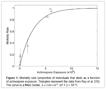
Figure 1: Mortality rate (proportion of individuals that died) as a function of actinospore exposure. Triangles represent the data from Ray et al. [15]. The curve is a fitted model;  .
.
The estimated per-fish infection rate per concentration of actinospores is shown as a function of temperature (Figure 2). First, the infection rate at 13°C was estimated and plotted as a horizontal line at the lower part of temperature. Then, a quadratic function was fitted to the infection rates at 15°C, 18°C, and 21°C.
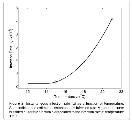
Figure 2: Instantaneous infection rate (α) as a function of temperature. Stars indicate the estimated instantaneous infection rate  , and the curve is a fitted quadratic function extrapolated to the infection rate at temperature 13°C
The effect of stream discharge on the mortality rate is shown in Figure 3. In this analysis, it was assumed that fish were exposed to actinospores over 24 hours at 18°C and the discharge alone varied according to the estimated discharge. Results show that mortality rate fluctuation was larger in June than in September, but these fluctuations were smaller than the difference between the mean rates in June and September. The estimated coefficients, b6 and b9, were 1.1×10⁹ (σ2 : 2.9 × 10¹¹) and 2.4 × 10⁷ (σ2 :9 × 10⁸) respectively.
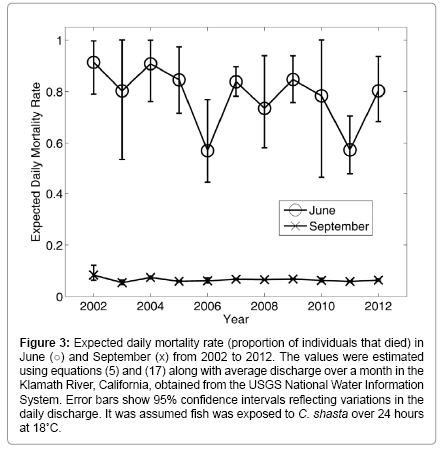
Figure 3: Expected daily mortality rate (proportion of individuals that died) in June (o) and September (x) from 2002 to 2012. The values were estimated using equations (5) and (17) along with average discharge over a month in the Klamath River, California, obtained from the USGS National Water Information System. Error bars show 95% confidence intervals reflecting variations in the daily discharge. It was assumed fish was exposed to C. shasta over 24 hours at 18°C.
Finally, Figure 4 shows the finite mortality rate of fish exposed to actinospores over a 24-hour period as a function of temperature and discharge. For a given discharge and temperature, the mortality rate in June was much higher than that in September.
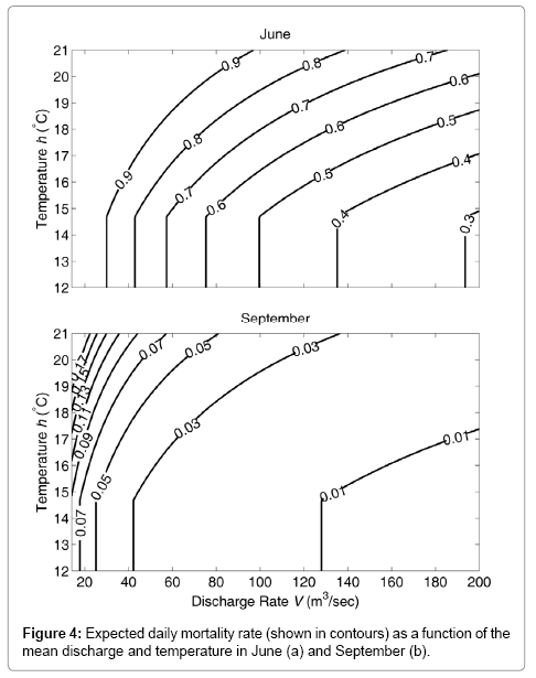
Figure 4: Expected daily mortality rate (shown in contours) as a function of the mean discharge and temperature in June (a) and September (b).
The sensitivities of the mortality rate to the duration of exposure, discharge, and temperature were calculated around the estimated values obtained for June and September 2008. Table 3 shows the sensitivity values and their inverses, the latter of which reveal the relative amount of change in a given condition needed to increase the mortality by a unit amount. Their relative magnitudes suggest that increasing the discharge by 1 m3/sec in June had an effect equivalent to that of decreasing the exposure duration by 0.26 hours or decreasing the temperature by 0.053°C. In September, increasing the discharge by 1 m3/sec had an effect equivalent to that of decreasing the duration by 0.73 hours or decreasing the temperature by 0.15°C.
| Parameters | Sensitivity |
Inverse of sensitivity  |
Sensitivity  |
Inverse of sensitivity  |
|---|---|---|---|---|
| June | September | |||
| Exposure Duration (I) | 0.0147 | 68.2 | 0.0027 | 377.0 |
| Discharge (V) | -0.0039 | -258 | -0.0019 | -517 |
| Temperature (h) | 0.0735 | 13 | 0.0133 | 75 |
Table 3: Sensitivities of the mortality rate (% death) to exposure duration, discharge, and temperature. Sensitivities and the inverse of the sensitivities are shown. These values were evaluated with the estimated parameters for June and September 2008. See text for detail.
The novelty of the study was its development of mathematical models based on existing C. Shasta data and extracting information useful for the management of Chinook salmon. Data for the study were primarily obtained from Ray et al. [14,15]. Each model was developed separately for different environmental factors, but could be integrated into equation (5) to model the overall mortality rate of Chinook salmon. This, in turn, could be incorporated into a population model for Chinook salmon [17]. To my knowledge, a development of the model that allows the integration of various environmental factors into a single unifying model for the parasite-induced mortality of fish is new. Finally, the models can be used to analyze the sensitivity of salmon mortality rates to environmental conditions, which is expected to be especially useful for future salmon management.
The persistence of C. Shasta requires two hosts: salmon and polychaete. Both juvenile salmon migrating downstream in spring and summer and adult salmon migrating upstream in fall are infected with actinospores of C. Shasta through their gills [13]. If the host dies after infection, myxospores of C. Shasta are released into the water. The myxospores later infect polychaetes. Because of delay in the death of salmon after infection and the directions of fish migration, I suspect that adult salmon are more important in releasing the myxospores, which infect polychaete, but further research is needed to confirm this hypothesis. The concentration of actinospores in the water is a very important determinant of the infection rate of salmon by the parasite [16]; this is consistent with the fact that the infection takes place through the gills. Unfortunately, the life cycle of polychaetes is not well understood [20]. If further information becomes available, however, it can be incorporated into the release rate of actinospores (κ) in equation (6). Ultimately, the release rate κ can be a function of the rate of release of actinospores per polychaete, the density of polychaete, and the discharge of water. The first two rates can also be a function of environmental conditions.
The rate of successful infection was found to increase with temperature [14]. In the present study, this effect was quantified in terms of the instantaneous rate of successful infection αh (Figure 2). The water temperature in the upper Klamath River currently ranges from below 5°C in winter to above 20°C in summer months [22]. According to the comparison of the estimated infection rate versus temperature (Figure 2), the increase in infection rate with increasing temperatures appears to accelerate within the higher temperature range. River temperatures in April and May, when numerous juvenile salmon typically pass through the infectious zone, is within this range. Furthermore, the sensitivity analysis suggests that the same amount of temperature changes has a greater effect on salmon mortality rate in June versus September (Table 3). This suggests that spring temperatures may contribute to determining the number of salmon surviving the infectious zone.
Ray and Bartholomew [16] showed that the total infection rate increases with temperature from 11°C to 18°C but declines from 18°C to 22°C. This appears to contradict with the results shown in Ray et al. [14]. However, the difference between the results from Ray et al. [14], the results presented herein, and the results from Ray and Bartholomew [16] is that the former quantifies the effect of temperature on salmon mortality, while the latter quantifies the effect of temperature on the number of transmissions of C. Shasta to salmon. Not all infections of salmon with parasites lead to the subsequent death of salmon [14]; therefore these results cannot be compared directly. Both studies, however, suggest the mortality rate per parasite after infection increases substantially with temperature although the total infection rate may decline. At temperatures above 18°C, the rate of successful infection (α) is expected to accelerate with the total infection rate (γ), and the results in Ray and Bartholomew [16] can be incorporated into changes in the total infection rate.
Bjork and Bartholomew [13] reported that the infection rate (γ) is affected by the velocity of water. It should be noted that the infection rate (γ) is the instantaneous rate at which actinospores enter salmon per actinospore concentration and salmon density. In the current study, this quantity was assumed to be constant regardless of the temperature and discharge. However, the effect of water velocity on infection rate is difficult to investigate. For example, the velocity could affect the amount of water filtered by salmon, which would affect the total exposure of salmon to the parasites. The velocity could also affect physical infection processes in fish gills. These processes, however, are confounded with the behavior of fish. For example, in a caging experiment, fish remained in a cage against water flow, but naturally swimming salmon might actually be carried with the flow or actively swim downstream [26]. If more detailed information on the effect of velocity on infection rate (γ) becomes available in the future, it would be interesting to incorporate it into the model.
There are clear differences in the mortality rate between June and September (Figure 4). The water temperature of the Klamath River is generally higher in September versus June, while the discharge is lower in September versus June. Both of these observations suggest that the parasite-induced mortality rate should be higher in September than in June. However, the estimated mortality was much higher in June versus September, regardless of the temperature and discharge. Therefore, the between-month difference in mortality cannot be explained by the effect of temperature on the development of C. Shasta after infection or the effect of discharge on the concentration of actinospores in the water. Instead, the difference is explained by the difference in the concentration of actinospores in the water [15]. This suggests that the natural mortality rate of actinospores (δ ), their release rate from polychaetes (κ), and/or the infection rate (γ) differed substantially between the two months according to equation (8). This, in turn, suggests the importance of studying polychaete life cycle and actinospore mortality rate in order to understand the observed seasonal difference.
An important assumption in the model is that all juvenile salmon have the same susceptibility to actinospore infection. It is plausible that there is heterogeneity in susceptibility. If so, one way to incorporate such heterogeneity would be to make the infection rate, α, include individual heterogeneity. It is also plausible that hatchery-released and naturally spawned juveniles may have different susceptibilities. Such heterogeneity could be incorporated into mathematical models by dividing the juveniles into two groups and separately estimating their parameters.
The sensitivities of the mortality rate to the temperature, discharge, and exposure duration were calculated, but direct comparison was difficult because the environmental variables had different units. Therefore, the inverse of each sensitivity was taken in order to calculate the unit change in a given environmental condition that was required to change the mortality by the same unit amount. Although the changes in salmon mortality may appear to be very small, the abundance of juvenile salmon is high. Therefore, a small change in the mortality rate can translate into a large difference in the number of salmon surviving the infectious zone. The sensitivity results can be used in planning for the restoration or mitigation of salmon habitats. Discussions are currently underway regarding the removal of dams from the Klamath River, which would be expected to change the flow pattern and water temperature. This sensitivity analysis can be used to predict the effects of these changes on the mortality of Chinook salmon from C. Shasta infection.
The primary goal of this study was to build models and parameterize them with existing data, in order to understand the mortality of juvenile Chinook salmon resulting from the infection with C. Shasta. The results are constrained by the limited availability of data, but the basic model structures should be very useful for managing environmental conditions in the Klamath River and predicting the future conditions that will be seen following the removal of dams. The utility of these novel models should improve in the future, as more data are collected, allowing us to predict responses resulting from future environmental conditions.
I thank three anonymous reviewers and editor, who provided very constructive comments and suggestions on the previous version of the manuscript. I also thank Cyrenea Piper for assisting the preparation of this paper. This research was made possible through support provided by the U.S. National Oceanic and Atmospheric Administration, National Marine Fisheries Service (DOC Contract- NFFR7500-10-18114). The opinions expressed herein are those of the author and do not necessarily reflect the views of the funding agency.