Journal of Glycomics & Lipidomics
Open Access
ISSN: 2153-0637
ISSN: 2153-0637
Research Article - (2015) Volume 5, Issue 2
This article presents multi-layered basic research culminating in what we call the Master Code of Biology. First, we review the “Formula for Life” discovery. This simple formula unifies all the components of life, structuring them in a kind of “Periodic table of Biology”. These components include bio-atoms, CONHSP, nucleotides, UTCAG, amino acids, DNA and RNA strands, proteins, genes, chromosomes and genomes. This discovery opens the door to powerful insights in exobiology, proposing a specific life-emerging constraint on the tuning and balancing of isotope proportions. Second, we introduce the “Master Code of Biology”, digital language supplying a common alphabet to the three fundamental languages of Genetics, Biology and Genomics. This synthesis goes above and beyond their three representative DNA, RNA and amino acids codes. There is a universal common code which unifies, connects and contains all these three languages. This “Master Code of Biology” provides a great Unification between the Master Code patterned images of Genomics (DNA) and Proteomics (amino acids), which appear highly correlated while RNA images curiously appear flat like a neutral or zero-like code. Third, the functionality of this discovery is evidenced by two examples. Analyzing textures of the Genomic and Proteomic patterned curves reveals the emergence of binary codes and discrete waveforms. These predict the well-known karyotypes- white/grey/black bands overlapping and characterizing the human chromosomes. Mapping “the Master Code of Biology” to SNP genomic areas, we show that SNPs are determined to be more functional by their location within the genome than by their local values– TCAG nucleotide changes. Finally, we demonstrate that a chromosomal DNA sequences systematic reshaping combined with periodic waves highlighted above brings out, at whole chromosome scale, interferometry-like interference fields manifested by resonances, tunings, and even resonances that exhibit Fibonacci number proportions differentiating human and great primates at whole chromosome4 scale.
<Keywords: Universal genetic code; Human genome; Genomics; DNA decoding; Nested codes; Information theory; Evolution; SNP; Origins of Life; Exobiology; Fractal genome; Golden ratio; Fibonacci numbers; Resonances; Interferences fields
We have been studying numerical structures in DNA and genomes for about 25 years [2-4]. We now present significant results from a 1997 discovery that was explored and developed over the last fifteen years1. The most comprehensive descriptions to date are found in the book [5,6].
Initially our main goal was to understand the heterogeneity of the two languages of DNA and amino acids linked by the heterogeneous universal genetic code table. A number of researchers are working in this difficult yet important field [7-12].
How is it possible to discover a law unifying two worlds as different as DNA codons and amino acids? We discovered three candidates that may link and possibly unify these two worlds.
I. First, atomic mass provides a common measure of codons and amino acids that are built with common bio-atoms.
II. Second, envisioned a law of digital projection of the atomic masses that could provide periodicities and regularities. Indeed, a phenomenon which appears heterogeneous in a tridimensional space can emerge regular and organized when the same data space is analyzed in two dimensions.
III. Third, we had a hunch that the universal variables like Pi and the golden ratio Phi [13] might play a role in this projection formula.
It is the synthesis of these three intuitive tracks that lead to the discovery of this formula. It unifies all the molecules of life, and we call it “The Formula for Life.” Since 1997, this discovery has been improved across multiple segments of biology, genetics and genomics. These results have been only partially published [13-17] and in the drafts [18- 20]. Our central discovery (methods and algorithms) will be now fully revealed in this article then in a series of others in preparation [21-24].
Genome analyzed
We analyzed the whole human genome in its most recent release [25,26].
Bravais-Pearson Correlation Method
All correlations in this paper run the “Bravais-Pearson” linear correlation coefficient algorithm [27].
Now2, we present the “Master Code” Discovery, detailing it in 4 steps:
• Formula for Life
• The Periodic Table of Biology
• Biology Master Code
• Discrete Waveforms and Logic Biobits
A summarized overview of these 4 breakthroughs is presented in the 4 next paragraphs.
An overview on formula for life discovery
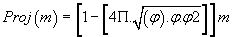
A quick presentation of the formula for life: In [5,6,14,15] we introduced the law we call Formula for Life. This law unifies all of the components of living including bio-atoms, CONHSP and their various isotopes, to genes, RNA, DNA, amino acids, chromosomes and whole genomes. This law is the result of a simple non-linear projection formula of the atomic masses. The result of this projection is then organized in a linear scale of integer number based codes (e.g., -2, -1, 0, 1, 2, 3...) coding multiples Pi/10 regular values. These codes are called Pi-masses.
Computing the “Formula for Life” associated with any atomic mass of Life components:
For atomic mass of any biological compound, we operate the “projection” of the atomic mass numerical value using the following operator:
 (1)
(1)

The result is a real number which we retain only the residues (decimal remainder).
Detailing the “PPI (mass)” projection: Consider any atomic mass « m », which may be that of a bio-atom, of a nucleotide, a codon of an amino acid or other genetic compound based on bio-atoms or even, any atoms (Mendeleiëv Table, [21]).
This process will work especially on the average masses (Table 1). But it may also be applied to a particular isotope or any derivative of specific atomic mass proportions of the various isotopes.
| Nature | Molecule or bioatom | Average atomic mass | Projection PPI(m) | Pi-mass NPI(m) = N.Pi/10 |
Angle | Error EPI(m,N) |
|---|---|---|---|---|---|---|
| Bioatom | C12 Carbon isotope 12 | 12.000000 | 0.01441631887 | 0 PI/10 (0°) | 0° | 0.01441631887 |
| Bioatom | C (Carbon average mass) | 12.0111 | 0.0003703460363 | 0 PI/10 (0°) | 0° | 0.0003703460363 |
| Nucleotide | G (G nucleotide) |
150.120453 | 0.01974469326 | 0 PI/10 (0°) | 0° | 0.01974469326 |
| Codon | Codon TCA | 369.324471 | 0.01106361166 | 0 PI/10 (0°) | 0° | 0.01106361166 |
| Codon | Codon UCA | 355.297477 | 0.6968708101 | -1 PI/10 (-18°) | -18° | 0.0110300755 |
| Codon | Codon AGT (TCA complement) | 409.349065 | 0.6930222208 | -1 PI/10 (-18°) | -18° | 0.0071814862 |
| double-stranded DNA | DNA double strand : TCA+AGT | 778.673536 | 0.7040858325 | -1 PI/10 (-18°) | -18° | 0.0182450978 |
| Amino acid | PRO (Proline amino acid) | 115.13263 | 0.6281423922 | +2 PI/10 (+36°) | +36° | 0.0001761385 |
| Amino acid | LYS (Lysine amino acid) | 146.190212 | 0.2553443926 | +4 PI/10 (+72°) | +72° | 0.0012926688 |
| Peptide link | CONH Peptidic link | 43.025224 | 0.6847234457 | -1 PI/10 (-18°) | -18° | 0.0011172889 |
| Notes: Projections PPI(m) are multiples of Pi:10. Example: 0.314... = 1Pi/10, 0.628... = 2Pi/10, etc... But, symmetrically vs. 0Pi/10, it appears another regular scale of attractors in the negative region of Pi/10: -1Pi/10 = 1-0.314 = 0.685..., -2Pi/10 = 1-0.628... | ||||||
Table 1: A set of Pi-mass projections for some main Life compounds.
 (2)
(2)
where 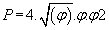 (3)
(3)
then P = 0.742340663...
Now, consider the “v” value, where v is always a negative or zero real number.
Then consider the function:
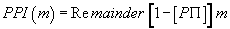
 (4)
(4)
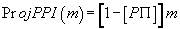
Where Abs (v) is the absolute value of v, and « remainder » or « residue » the decimal remainder of the numerical projection
For example: remainder (-27.85) = 28-27.85 = 0.15
We then defined PPI (m) such that:
 (5)
(5)
Note that (1-P.PI) is always negative because m is always positive, and (1-P.PI) is always negative.
As an example, consider the amino acid GLY:
We defined the average mass of GLY as: GLY = 75.067542
Then: (1-P.PI) . GLY = -99.99987286
Thus, PPI (GLY) = remainder [(1-P.PI) . GLY] = 0.0001271351803
Or, finally, PPI (GLY) = 0.0001271351803
Although no longer considered the decimal part, we note that, if we were interested in the set
(1-P.PI) . GLY = -99.99987286, this value is substantially equal to 100 = 10*2 ... which is not “just any number” ... So then, what is the geometric reality of this projection? As Figure 1a summarizes below, everything happens as if the atomic mass was “filtered” through the competitive interference of two projections: one through a cube of side = 1 and the second through of a sphere of radius = φ × 7/4.

Figure 1: (a) “Formula for Life” non linear projection highlights reveals a regular projection scale based on Pi/10 units. (b) “The Periodic Table of Biology”: evidence of a regular projection scale based on Pi/10 units. (c) Fine-tuned selectivity of the “Formula for Life” comparing average atomic mass with light and heavy single isotopes masses
Table 1 below illustrates the calculation of Pi-mass projections for some representative biological components: bioatoms, nucleotides, DNA codons, amino acids.
An overview of the “Periodic Table of Biology” discovery
In Figure 1b, we introduced to 162 Genetic Code and organic compounds representing biological components. In one hand, the real atomic masses and, on the other hand, their corresponding Pi-mass weights projections. This figure then reveals the “periodic” nature of these regular patterned projections. We note that the two increasing areas to the right of the graph correspond to the respective curves of the 64 DNA and RNA codons atomic weight.
We call Table 2 the “Periodic table of Biology”: It represents successive regular periods based on Pi/10 tokens. It shows all the essential components of Biology and Genetics: bioatoms, DNA and RNA nucleotides, amino acids, codons and codon pairs from DNA and RNA molecules.
| Period | Nature | Example | Atomic Mass | Pi-mass | Angle | Error |
|---|---|---|---|---|---|---|
| 1 | Isotopes | Carbon C12 | 12.00000 | 0 Pi/10 | 0° | 0.014416327 |
| 2 | Average atomic mass | Carbon atom | 12.01110 | 0 Pi/10 | 0° | 0.000370338 |
| 3 | Simple molecules | H2O | 18.0153240 | 0 Pi/10 | 0° | 0.001210900 |
| 4 | Complex molecules | Codon TCA | 369.324471 | 0 Pi/10 | 0° | 0.01106361166 |
| Notes: It will be noted that compounds of very different weights may have the same Pi-mass projection. | ||||||
Table 2: ”The Periodic Table of Biology”, suggesting a biomolecule complexity vertical Period dimension.
Is it legitimate to speak of “Periodic Table of Biology” by analogy with the universal “periodic table” of Mendeleev? We say yes, for the following two reasons:
First the regular pitch multiples of Pi/10 define, in our view, the horizontal dimension of the table (horizontal column size).
On the other hand, to complete the Mendeleïev’s table analogy, on the vertical scale, the periods vertical size in the table of Mendeleïev could be formed by the levels of complexity of the molecules.
Thus, period one would be that one of the isotopes, period two the average atomic masses of atoms, period 3 simple molecules, and period 4 complex composite molecules.
Table 2 below suggests an example of four periods (lines) on the Pi-mass = 0 column. Finally, to complete the analogy, we will show in [22] how we can associate a kind of simple algebra and allowing combinatorial, analytically calculate Pi-mass directly from the 6 basic CONHSP Pi-mass bioatoms.
An interesting research track of this “Period dimension” is that of a possible link between these molecules with same Pi-masses and their possible tri-dimensional shape: In fact, two contiguous molecules with same Pi-mass could control the geometric orientation of successive spatial planes organization. Thus, the molecules gradually increase assembly complexity, whether both cases of the same or different single molecules or very different complexities molecules - for example interaction between a DNA codon and a water molecule (Table 2).
A startling observation opens the door to enormous opportunities in astrobiology: Table 3 and Figure 1c shows a very curious fact: the Pi-mass projection formula seems optimal only for the atomic masses of average atomic weights of basic life bioatoms C O N H. Instead of tiny perturbations on these atomic masses and atomic masses of the individual isotopes (example O16) of each of these atoms “destroy” the optimality and fine-tuning of these projections then, also, consequently all resulting master code perfect tuning. Example here (Table 3) for the Pi-mass projection of Oxygen isotopes and % average weighted atom mass. As shown in Figure 1c, isotopes of oxygen lightest and heaviest O16 O18 both produce an error on the projections Pi-mass much higher than that of the average atomic mass of that atom of oxygen consisting of: 99,757% + 0.04% O16 O17 + 0.2% O18.
| Atom | Isotope | Relative atomic mass | % isotopic composition | Pi projection residue and Pi mass value | Pi-mass NPI(m) = N.Pi/10 | Error EPI(m,N) |
|---|---|---|---|---|---|---|
| Oxygen | Average % balance |
15.9994(3) | - | 0.686647751 0.685840735 | -1 | 0.000807016 |
| O16 | 15.994 914 619 56(16) | 0.997 57(16) | 0.692662834 0.685840735 |
-1 | 0.006822099 | |
| O17 | 16.999 131 70(12) | 0.000 38(1) | 0.354913152 0.371681469 |
-2 | 0.016768318 | |
| O18 | 17.999 161 0(7) | 0.002 05(14) | 0.022742056 0.000000000 |
0 | 0.022742056 | |
| Notes: 0.685840735 = 1 – Pi/10, 0.371681469 = 1 – 2Pi/10 | ||||||
Table 3: Example of Pi-mass projection fine-tuned selectivity for Oxygen average mass vs. individual isotopes
To summarize, we discovered a formula unifying ALL biological components from C O N H S P bioatoms to DNA, RNA, amino acids and then genes proteins chromosomes and genomes. But this perfect balance is optimal only when atom atomic mass is the % mix from our Earth atmosphere: i.e., % C12 C13 C14, etc.
This fine tuning is destroyed by example when all isotopes are only C12, and also in case of environmental disasters. For example, the proximity of a large chemical plant alters the relative proportions of isotopes of carbon or oxygen. This results in an imbalance of the Pimasses and consequently embrittlement of DNA [23]. This can induce cancers through chromosomal translocations.
What is the reason that the perfect selectivity of our «formula for Life» which in fact are operational only when the relative proportions of bio-isotopes are exactly those that we measure in our Earth’s atmosphere, inherited from millions of years of evolution [28]?
The main question now is: Is this perfect balance of isotopes proportions the result of Earth and atmosphere evolution according to the thesis of Dr. James Lovelock [29]?
In [5] I sketched an alternative hypothesis: The multiple isotopes of the same atom are perhaps only partial views of multi-isotope atoms. By analogy, consider how white light is a synthesis of multiple components of basic spectral colors. Here, the phenomenon is similar but opposite in kind… This again would mean that the true atomic weight is the average atomic mass of the atom, all isotopes together, while individual atomic masses of each isotope would be only “partial views” of this global and multi-isotope atom. The reasons for this possible multi-isotope perception could be of quantum nature [30].
The new question now is: « Is this the result of James Lovelock’s GAIA theory? Or, perhaps isotopes don’t exist but are quantum views of a meta-multiple-isotope-quantum-atom-structure? »
A strong consequence for Exobiology: The atmosphere-like percentage balancing and mixing of isotopes is a prerequisite within CONH bio atoms and is a necessary, but not sufficient - condition for earth like Life on other planets.
More specifically: “The emergence of life requires the existence of specific proportions of different isotopes of each of the 4 bio atoms–C (carbon) O (oxygen) N (nitrogen) H (hydrogen)–such that the balance between these proportions (C12 / C13, O16 / O17 / O18, N14 / N15 and H1 / D) is strictly identical to that observed in the Earth’s atmosphere.”
Finally, in [5] in Chapter 20, we show how this superior Pi-mass based average atomic mass compared to Pi-mass of basic isotopes, can be extended to thousands of organic molecules referenced in the famous Beilstein3 dictionary: we study the primitive molecules of the astrobiology to complex living components, also passing by thousands of molecules of organic chemistry.
An overviev on the “Biology Master Code” Great Unification of DNA, RNA and Amino acids
It may seem surprising that such a fine tuned process like biology of Life requires the use of three languages as diverse and heterogeneous as DNA with its alphabet of four bases TCAG; RNA with its alphabet of four bases UCAG; and proteins with their language of 20 amino acids. Obviously, the main discoveries in biology were made by those who managed to unearth the respective areas and “bridges” between these three languages. However, any “aesthete” researcher will think the table of the universal genetic code seems rather “ad hoc” and heterogeneous.
Starting only from the double-stranded DNA sequence data, the “Master Code” is a digital language unifying DNA, RNA and proteins that provide a common alphabet (Pi-mass scale) to the three fundamental languages of Genetics, Biology and Genomics.
The construction method of “the Master Code” will be now fully described below. It will highlight a significant discovery we summarize as follows: “Above the 3 languages of Biology - DNA, RNA and amino acids, there is a universal common code that unifies, connects and contains all these three languages”. We call this code the “Master Code of Biology.”
Here is a brief description of our process for computing the Master Code:
The coding step: First, we apply it to any DNA sequence encoding a gene or any non-coding sequence (formerly mislabelled as junk DNA). So it may be either a gene, a contig of DNA, or an entire chromosome or genome. In this sequence, we always consider double-stranded DNA as we explore the following three codon reading frames and following the two possible directions of strand reading (3’ ==> 5’ or 5’ ==> 3’). The base unit will always be the triplet codon consisting of three bases.
As shown in above sample, we calculate the Pi-mass related to double stranded triplets DNA bases, double stranded triplets RNA bases, and double-stranded pseudo amino acids. In fact, for each DNA single triplet codon, we deduce the complementary Crick Watson law bases pairing. We do the same work for RNA pseudo triplet codon pairs, then, similarly for amino acids translation of these DNA codon couples using the Universal Genetic Code table. Then we obtain 3 samples of pairs codes: DNA, RNA and amino acids and this, systematically even when this DNA region is gene-coding or junk-DNA.
A simple example: the starting region of Prion gene:
DNA image coding:
ATG CTG GTT CTC TTT...
-1 -1 -1 0 0...
Complement:
TAC GAC CAA GAG AAA...
0 -1 0 -2 0...
RNA image coding:
AUG CUG CUU CUC UUU...
-2 -2 -3 -1 -3...
Complement:
UAC GAC GAA GAG AAA...
-1 -1 0 -2 0...
Proteomics image coding:
MET LEU VAL LEU PHE
4 3 3 4 3...
Complement:
TYR ASP GLN GLU LYS
2 -1 1 0 4...
Pi-masses corresponding to two strands are then added for each triplet:
Double strand DNA image coding: -1 -2 -1 -2 0...
Double strand RNA image coding: -3 -3 -3 -3 -3...
Double strand Proteomics image coding: 6 2 4 4 7...
This produces three digital vectors relating to each of the 3 DNA, RNA, and proteomics coded images.
This produces three digital vectors relating to each of the 3 DNA, RNA, and proteomics coded images. At this point we already reach an absolutely remarkable result, as symbolized in Figure2a

Figure 2: (a) “Master code of biology” and Great Unification shows an equivalence of both Genomics (DNA) and Proteomics (amino acids) signatures while the RNA signature is a neutral area like a “zero”. (b) A typical correlation between Genomics and Proteomics signatures related to the Prion protein, the whole Malaria chromosome 2, and the whole HIV1 genome.
The coded image of any RNA sequence is “flat” (always=-3) and monotonic, and can be likened to the “zero” or “neutral element of Biology”!
We will focus now – exclusively - on the DNA code (genomics) and amino acids code (proteomics).
The globalization and integration step: To these two numeric vectors we apply a simple globalization or integration linear operator. It will “spread” the code for each position triplet across a short, medium or long distance, producing an impact or “resonance” for each position and also on the most distant positions, reciprocally by feedback. This gives a new digital image where we retain not the values but the rankings by sorting them.
We run this process for each codon triplet position, for each of the three codon reading frames and for the two sequence reading directions (3’ ==> 5’ and 5’ ==> 3’).
For example, to summarize this method: on starting area of the GENOMICS (DNA) code of Prion above, the “radiation” of triplet codon number 1 would propagate well:
-1 -2 -1 -2 0... ==>
-1 -3 -4 -6 -6...then, we cumulate these values: -20
So we made a gradual accumulation of values.
The same operation from the codon number 2 produces:
-1 -2 -1 -2 0... ==>
-2 -3 -5 -5...then, we cumulate these values: -15 4
etc.
Similarly, the same process on starting area of the PROTEOMICS code of Prion above, the “radiation” of triplet codon number 1 would propagate well:
6 2 4 4 7... ==>
6 8 12 16 23...then, we cumulates these values: 65
So we made a gradual accumulation of values.
The same operation from the codon number 2 produces:
6 2 4 4 7... ==>
2 6 10 17...then, we cumulate these values: 35 5
etc.
Finally, after computing by this method these “global signatures” for each codon position at Genomics and Proteomics levels, we sort each genomic and proteomic vector to obtain the codon positions ranking: example: as illustrated bellow, the Genomics ranking patterned signature is 2 1 4 3 5 for this Prion starting 5 codons mini subset sequence of 5 codons positions (arbitrary values). Then, to summarize the Master Code computing method on these 5 codon positions starting Prion protein sequence:
Genomics signature:
Codon 1:
Codon / Basic codes / Potentials (with circular closure) / circular complements:
!
-1 -2 -1 -2 0
-1 -3 -4 -6 -6
0
Cumulates: -20
Codon 2:
Codon / Basic codes / Potentials (with circular closure) / circular complements:
!
-1 -2 -1 -2 0
-2 -3 -5 -5
-6
Cumulates: -21
Codon 3:
Codon / Basic codes / Potentials (with circular closure) / circular complements:
!
-1 -2 -1 -2 0
-1 -3 -3
-4 -6
Cumulates: -17
Codon 4:
Codon / Basic codes / Potentials (with circular closure) / circular complements:
!
-1 -2 -1 -2 0
-2 -2
-3 -5 -6
Cumulates: -18
Codon 5:
Codon / Basic codes / Potentials (with circular closure) / circular complements:
!
-1 -2 -1 -2 0
0
-1 -3 -4 -6
Cumulates: -14
Final rankings:
Codon positions: 1 2 3 4 5
Potentials: -20 -21 -17 -18 -14
Rankings: 2 1 4 3 5
Then we run similar computing for Proteomics...
Codon 1:
Codon / Basic codes / Potentials (with circular closure) / circular complements:
!
6 2 4 4 7
6 8 12 16 23
0
Cumulates: 65
Codon 2:
Codon / Basic codes / Potentials (with circular closure) / circular complements:
!
6 2 4 4 7
2 6 10 17
23
Cumulates: 58
Codon 3:
Codon / Basic codes / Potentials (with circular closure) / circular complements:
!
6 2 4 4 7
4 8 15
21 23
Cumulates: 71
Codon 4:
Codon / Basic codes / Potentials (with circular closure) / circular complements:
!
6 2 4 4 7
4 11
17 19 23
Cumulates: 74
Codon 5:
Codon / Basic codes / Potentials (with circular closure) / circular complements:
!
6 2 4 4 7
7
13 15 19 23
Cumulates: 77
Final rankings:
Codon positions: 1 2 3 4 5
Potentials: 65 58 71 74 77
Rankings: 2 1 3 4 5
Then finally:
Codon position: 1 2 3 4 5
Genomics vector: 2 1 4 3 5
Proteomics vector: 2 1 3 4 5
To complete, the same work must be also operate on each codon reading frame...
Meanwhile, a more synthetic means to compute these “long range potentials” for each codon position is the following formula:
Cumulate potential of codon location “i”
 (6)
(6)
Then, finally
 (7)
(7)
Example for Genomics image of codon “i”
The initial computing method described above provides:
-1 -2 -1 -2 0... ==>
-1 -3 -4 -6 -6...then, we cumulate these values: -20
becomes, using this new generic formula:
(-1)x5 + (-2)x4 + (-1)x3 +(-2)x2 +(0)x1 = (-5) + (-8) + (-3) + (-4) + 0 = -20
The great Unification between Genomics and Proteomics Master Code images: When applying the process described above in any sequence – gene coding, DNA contig, junk-DNA, whole chromosome or genome - a second surprise appears just as stunning as that of RNA neutral element. We find that for one of the three reading frames of the codons given, the Genomics patterned signature and the Proteomics patterned signature are highly correlated.
Contrary to the three genomics signatures which are correlated in all cases, the proteomics signatures are correlated with genomics signatures only for one codon reading frame, and generally in dissonance for the two remaining codon reading frames. Also, there are perfect local areas matching’s focusing on functional sites of proteins, hot-spots, chromosomes breaking points, etc.
Figure 2b summarizes this universal breakthrough for the general case and for three representative cases: Prion protein [31], a whole chromosome of Malaria disease, and a complete HIV1 genome [24]. It is important to note the universal character of this coupling of genomics/proteomics: for example, for some three billion base pairs of the whole human genome, we have verified this law across the entire genome, for all its chromosomes and in all its regions with a global correlation of about 99%.
In this global correlation, specific codon positions were a perfect match. This is remarkable when regions correspond to biologically functional areas: hot-spots, the active sites of proteins, breakpoints and chromosome fragility regions (i.e., Fragile X genetic disease), etc.
Towards discrete Waveforms and logic Biobits overlapping whole chromosomes and genomes
Here we analyze the texture, that is to say, the “roughness” of genomic and proteomic signatures provided by the Master Code. For this, we need only to analyze the slopes or mathematical differentiations from these patterned curves: slopes and gradients - in the sense of LEIBNIZ? - of order 1, order 2, of order n.
The curves of the Master Code are discontinuous (each point represents a position of triplet codon).
If we note M (i) the Master Code function as defined in §4.4, then we agree that:
slope = 1 = ”growing” i.e., “increase” if M (i + 1) > M (i)
and slope = 0 = “decreasing” i.e., “decrease” if M (i + 1) < M (i).
Biobits: The emergence of a “binary language” from the Proteomics Master Code of any DNA sequence:
A detailed analysis of the texture of Genomics and Proteomics curves reveals a strange phenomenon: as shown in Figure 3a, a curious roughness or “sawtooth” usually characterizes these images. This somehow amounts to a search for the “derivative of order 1”, that is to say the slope between two successive points. It becomes apparent that these slopes are mostly in the same direction: always growing or always decreasing. Here is a small example of a sequence of 312 bases where genomics (blue) and proteomics (green) signature (amino acids) are studied. Note the beauty of these mathematical structures which always increase and that some compare to artistic works by M.C. Escher or J.S. Bach.

Figure 3: (a) “Master Code” typical derived increasing slopes of the proteomics patterned signature. (b) Human chromosome 22 Proteomics Binary code (blue) and Genomics Analogic code (brown). (c) Human chromosome 22 Attractors evidence: Proteomics Binary code (blue) and Genomics Analogic code (brown). (d) Human chromosome 4 Binary Attractors evidence of the Proteomics Binary code texture signature.
In the two other images below (Figure 3b and Figure 3c), we generalized this study to whole human chromosome 22 studied in its entirety. By convention, the sequence is segmented into small pieces (e.g., 10000 bases pairs) then we compute the total amount of “increase” type (growing) textures (increase %).The structures that we will discover are fractal because they stay self-similar for smaller segmentations 1000 base pairs, or larger than 100000, 1000000 bases pairs.
If this work is carried out for Genomic patterned pictures, we see that if this trend seems self-organized around one attractor for DNA double strand (Genomics), it shows two levels, two “attractors” for the second (Proteomics). A curious fact then emerges: although two genomics and proteomics curves are still highly correlated in their respective forms and shapes, we discover that their textures are radically different.
Thus the population of Genomics curves will be relatively dispersed around one single withdrawing attractor in a kind of Gaussian dispersion, while the population of Proteomic curves will be distributed around two attractors, bringing out a kind of binary frequency modulation.
We are witnessing the emergence, the “birth” of a Binary Code as demonstrated by Figures 3b, 3c, and particularly 3d!
Let us not forget that the initial information was the atomic mass of each bio-atom, which is... a real (decimal) number!
Then it is transformed into a code which is an integer number...
and it now emerges Binary Code, then 0/1 bits which are binary numbers!
Preliminary analysis shows that the average levels of these two attractors are around 0.61 (61%) and 0.30 (30%) then appear to be in a ratio of two. We will return to these two values bellow...
Discrete Waveforms: The emergence of “a modulated waveform code” from the Genomics Master Code of any DNA sequence:
The generalization of previous gradient differentiations from second, third or nth gradient differentiation order now highlight “bits”… But waveforms, more precisely discrete waveforms of which we will measure periods: period of short-wave or 2 or 3 or even medium-wave wavelengths (greater than 10 times).
Thus, we calculate exhaustively all successive gradients or slopes: S(i, i + 1), and S(i, i + 2), S(i, i + 3), ... S(i, i + n). From all these successive gradients periodicities emerge.
Figure 4a shows shortwave period = 4 codons, then 12 bases pairs in one million base pairs within human chromosome 3. Figure 4b shows long wave period = 12 codons, then 36 base pairs in the first 300000 base pairs within one of the largest human genes, the gene for the genetic disease Duchenne DMD.

Figure 4: (a) Evidence of discrete waveforms within 1 million bases pairs in human chromosome3. (b) Evidence of discrete waveforms within 300k-bases pairs from the DMD long Duchenne disease gene.
Functionality of Master Code Waveforms: the explanation of chromosomal alternated grey interferences bands
One of the experimental concrete chromosome representations is a universally known Karyotype image (Figure 5a).

Figure 5: (a) The Universal Human Genome chromosome banding called Karyotypes. (b) The Master Code Biobits and discrete waveforms provide a perfect prediction of Karyotype bands
However, the synthesis of two earlier codes (binary code and waveforms) allows prediction throughout the whole human genome of alternating black/gray/white bands of karyotypes! This is the clearest proof of the functional reality of our Master Code discovery. We must recall here that karyotypes are obtained by interferometry, physical process of wave nature.
Figure 5b is an illustration of the “calibration” in a portion of human chromosome 8.
In Figure 5b above, the green bars represent the actual referenced colors of the karyotype bands for this region of human chromosome 8: 0 = black, 1 = dark gray, 2 = medium gray, light gray = 3, and 4 = white. Blue curve, modulation of waves is predicted by the textures of the “Master code”: there is a fairly good correlation with the actual referenced colors of karyotypes, particularly, low wave period (2 or 3) for karyotypes clear (white), and waves heavy periods (in this case up to 16) for dark karyotypes (black).
Finally, Biobits, shown here in red, have a status = 1 = “increase” for karyotypes clear (white) and a status = 0 = “decrease” for dark karyotypes (black).
Such predictive analysis was performed for 24 chromosomes representing the entire human genome. The results show a perfect correlation between the predictions from the textures of the Master Code and grayscale karyotypes as they have been highlighted by the global community of geneticists [26]. Both Figures 6a and Figure 6b below show a graphical summary of texture modulations (Genomics) and Biobits (proteomics) throughout the whole human genome.

Figure 6: (a) Evidence of analogic modulated Genomics code (blue) and logic binary Proteomics code in human chromosomes 1 to 8. (b) Evidence of analogic modulated Genomics code (blue) and logic binary Proteomics code in human chromosomes 9 to Y
Notes:
-In each graph, the base unit analyzed X (horizontally) is one million base pairs long: there are 3266 units representing 3,266,000,000 bases pairs. Among them, 3.075 billion bases are significant, whereas the remaining 191,000,000 relate to GAPs (bases “N” indeterminate base pairs), in particular centromere regions of the chromosome.
-Vertical lines delimit the boundaries between each chromosome as centromere regions
-The two variations shown here correspond to DNA “Master Code” textures (Genomics) and amino acid like “Master Code” textures (Proteomics). They are computed independently for each of the millions of bases analyzed, or “one point” per million bases on the Genomics curve and “one point” per million bases on the Proteomics curve.
-The reader will note again here that although the variations of the Genomics and Proteomics curves are strongly correlated (96.63% on average over the whole genome), their “textures” are radically different!
This result is quite remarkable, showing both the fractal nature of the genome (roughness), and certainly an undulating wave-based nature of all genomic DNA. The reality and the evidence will probably be acknowledged within a few years [32].
In fact, the Genomics texture is “Analogically Modulated” around a region of about 60% mean value (6000 scale) would appear to be ... Fi = 1/Phi = 0.618.
On the contrary, the Proteomics texture (although strictly calculated using the same method and from strongly-correlated Master Code curves) is “Modulated In A Binary Logic,” continuously oscillating between two attractors whose respective values are: 30% = Floor average ceiling or 60% = Ceiling average. The relationship between these two attractors is very close to the number two. The scatter plot perfectly illustrates the reality of these two binary attractors 0 / 1 or “Floor / Ceiling”.
In fact, an analysis of these average values over the entire human genome [5] reveals this remarkable result
Average Ceiling values % = 0.618 = 1 / Phi
while average Floor values % = 0.309 = 1/2 Phi. So Ceiling / Floor ratio = 2.
Powerful applications for the Master Code of Biology: SNPs
The many potential applications of Master Code of Biology were discussed briefly in a few conferences and publications: principally, [18,31] and informal Web published drafts [18,20] describing the unification of the 3 languages of biology: DNA, RNA and amino acids chains. Here we show that the SNPs are more important and functional by their location within the genomic DNA sequence than by their nucleotide mutations! As illustrated by fractal embedded Russian dolllike Figure 7 In this context of synchronicity between 2 Genomics and Proteomics Master Code images, “peaks” and “valleys” will suddenly have functional significance. This is the case in the following 5 successive zooms around a specific SNP in the human genome (SNP AL391359 from chromosome 21). This strange property of SNPs was tested on large populations of SNPs: it shows that the SNPs, which are known to distinguish each individual vis-à-vis all other humans, are in their most important states in the position genome by the value of the change (e.g., T ==> A). In the following Figure 7, there are 5 successive nested zooms (Figure 7a to Figure 7e) in the same region of DNA located on either side of the SNP (vertical line). They will highlight the fact that the SNP was “nestled” exactly in a “hollow”. In other cases, it will nest on top instead of a “peak”. The reader can check the universality of this SNPs property in extending the study to other positions of SNPs, which we did exhaustively.

Figure 7: “Master Code” Evidence of the functional role of SNP location within the chromosomes DNA sequences: here the 5 embedded zooming sequences of 12000bp, 6000bp, 3000bp, 1500bp and 750bp centered around SNP
Let us now take a step back and consider the discoveries outlined above. We ask the reader to think a bit with us on each of the following four remarkable points. Here are the respective perspectives:
Exobiology
Self-organization
Information Theory
Code and reality
Then, we present a future perspective entitled
Future: Is the DNA sequence a Field of Interferences?
Exobiology perspective
It is absolutely remarkable that the original rule called “Formula for Life” is selective and sharp, becoming optimal when applied to the average atomic masses of bioatoms and basic components of life. Instead, its accuracy, fine-tuning and adjustment collapse when applied to a single isotope (O17 or O18 example) or the average atomic mass disturbed by an error (e.g., disturbance +/- 1/10000 [5]. This famous result then challenges the exobiology community on the isotopic balance of CONH bioatoms, which can be measured on other planets and as was done in November 2014, for the comet 67P / Churyumov- Gerasimenko. Did exobiologists discover the same mix of isotopes on these exoplanets? Or is this comet measuring our earth’s atmosphere? Indeed, we know that it is the activity of life which produces the isotopic balance in our atmosphere.
Self-organization perspective
In digital projection that has been discussed above, we consider the error adjustment of digital projections of atomic masses around multiple values of Pi/10. Thus (Table 4) will form - step by step - and by successive computation a real “periodic table of biological elements”. The whole of these Pi-Masses will now become integers, all multiples of Pi/10.
| Nature | -3Pi/10 | -2Pi/10 | -1Pi/10 | 0Pi/10 | +1Pi/10 | +2Pi/10 | +3Pi/10 | +4Pi/10 | 5 Pi/10 and +7Pi/10 |
|---|---|---|---|---|---|---|---|---|---|
| Bioatoms | P (-4pi/10) | H O | C | N | S | ||||
| Nucleotides | U G I | T C A | |||||||
| Annex Molecules | Phosphate/sugar RNA | CONH | H2O | CH2 Phosphate/ sugar DNA | |||||
| Amino Acids | Asp | Asn Glu Gly Ser | Ala Gln His Thr | Pro Tyr Cys (+2) | Arg Phe Trp Val | Ile Leu Lys Met (+4) | Cys (+5) Met (+7) | ||
| DNA Codons | ggg | gtg gcg gag tgg cgg agg ggt ggc gga | ttg ctg atg gtt gtc gta tcg ccg acg gct gcc gca tag cag aag gat gac gaa tgt tgc tga cgt cgc cga agt agc aga | ttt ttc tta ctt ctc cta att atc ata tct tcc tca cct ccc cca act acc aca tat tac taa cat cac caa aat aac aaa | |||||
| RNA Codons | uuu uug guu gug ugu ugg ggu ggg | uuc uua cuu cug auu aug guc gua ucu ucg gcu gcg uau uag gau gag ugc uga cgu cgg agu agg ggc gga | cuc cua auc aua ucc uca ccu ccg acu acg gcc gca uac uaa cau cag aau aag gac gaa cgc cga agc aga | ccc cca acc aca cac caa aac aaa | |||||
| Notes: a curious fact: DNA and RNA codons have negative or 0 Pi-masses meanwhile amino acids have positive or 0 Pi-masses. | |||||||||
Table 4: ”The Periodic Table of Biology” structuring ALL compounds of Life in a regular Pi/10 units scale
So after “digital and non-linear projection” of atomic masses, we see a genuine emergent process of self-organization. These classes of biological elements are all aligned and standardized around the integers -2, -1, 0, 1, 2, 3, etc., such that biological material will have the freedom of self-organization. Provided that these constraints are always respected, a set of “rails” is formed by these multiple integers of Pi/10. We then have a sort of open system, self-organized, yet highly constrained.
Information Theory perspective
The question raised by the Master Code of the Biology is very interesting to analyze in terms of information theory. Indeed, how could a double sequential set of defined codon triplets (codon triplets and complementary codon triplets) constituting the DNA double helix be found to encode in three distinct biological languages: DNA, RNA and amino acid languages?
A single common operator applied to each of these three suites will project three very remarkable images: the DNA image and the amino acids image lead to two-dimensional topologies that are highly correlated, as if the exact same thought had occurred through two distinct human languages such as English and Spanish, for example.
On the contrary, it is very strange that the RNA image always bring out – and we emphasize always - a flat topology and void, a neutral or “zero” element of Biology. Let us now turn to the roughness (the fractal sense) or the texture of both Genomics (DNA) and Proteomics (amino acids) topologies that are so strongly correlated at analogical values level i.e., the DNA image and the amino acids image.
They will then strangely differentiate: the Genomics texture distributing statistically and very diffusely around a mean value attractor 1/Phi = 0.618. Instead, the Proteomics texture will distribute in a very clean and binary fashion––two attractors around 1/Phi and 1/2 x Phi.
If we continue our analogy of a single thought communicated through two human languages (e.g., English and Spanish), suggesting that the strong differentiation between the two types of textures/ roughness corresponds with languages, sounds and speech with rich harmonic waveforms in both the musical and fractal sense.
Code and reality perspective
The considerations that follow are probably the most important fundamental results of this article. Indeed, consider the 24 pairs of chromosomes that comprise the human genome. Initially, we have a kind of Biological information, the double-stranded DNA sequence product of DNA sequencers outcome.
This information is a gift to biophysics and it is very “real”. What we have demonstrated in this article is that we can transform material information into completely Abstract Digital information. From this information - the Master Code of Biology - now emerges mathematical structures and a high-level of organized information such as discrete waves and binary codes.
Finally, we show that this abstract information is re-materialized in a real world measurement through the famous karyotypes that are the true identity of our genome map. Here, we still have waves from physical analysis of the chromosomes by Interferometry! So we travel back and forth between the biochemical reality of the mathematical image of the DNA molecule and finally, the reality of this materialized abstract digital image: karyotypes!
Finally, we can conclude with an excerpt from Pierre Teilhard de Chardin, The Phenomenon of Man [1]
“It is tiresome and even humbling for the observer to be thus fettered, to be obliged to carry with him everywhere the centre of the landscape he is crossing. But what happens when chance directs his steps to a point of vantage (a cross-roads, or intersecting valleys) from which, not only his vision, but things themselves radiate? In that event the subjective viewpoint coincides with the way things are distributed objectively, and perception reaches its apogee. The landscape lights up and yields its secrets.
He sees. That seems to be the privilege of man’s knowledge.” [1]
Future View: Is DNA sequence an Interferences Field?
Now let’s discuss the gradual emergence of global digital structures, then discrete waves and finally, digital interference field [33]. DNA sequence- could this be a kind of holographic memory of biological information?
Step 1: From local to global: In [34], the author reports the discussions between Albert Einstein and David Bohm about the quantum theory of Bohr. David Bohm proposes an interesting subquantum level concept called “quantum potential” where effects are not mitigated when the distance increases.
in § on the Biology Master code where we imagined “the globalization step”, we also wanted to spread the impact of each codon to all other codons forming the whole sequence and vice versa. Each codon is influenced by all other codon locations forming the sequence. So we have thus globalized mutual and reciprocal influences of all codon positions constituting the DNA sequence.
In [34], the author sums up quite well the whole point of globalization: “If you want to know Where You Are, ask a non-local”.
Returning for a moment about how we calculated the curves of “the Master Code” (The globalization and integration step). By this method, the Pi-mass codon “i” is propagated throughout the sequence and “the Master Code” influence of each of the other codons. As illustrated in the formulas below, this equates to a globalization of information and relocation of its influence and vice versa.
Potential cumulative developed codon “i”:
We recall that:
 (6)
(6)
Then, finally:
 (7)
(7)
Thus, the potential of the point “i” is the sum of n times the Pimass of this codon “i” + (n-1) times the Pi-mass of the next codon “i + 1” + (n + j) times the Pi-mass of codon “i + j”, ... / ... + once the Pi-mass of the previous codon “i-1”. Thus, the influence of all the codons of the sequence on the “i” address codon is linearly decreasing when advanced on the sequence which reminds us that it is considered looped back on itself.
All this potential for all codon positions (Genomics and Proteomics) thus provides a kind of two-dimensional topology composed by codon positions in x and by potentials in y. As we have stated previously, rather than potential curves, we retained their rankings, which is equivalent. This is how we built the curves of the Master Code such as those of Figures 2a and 2b.
Step 2: the emergence of numerical waveforms: This is the analysis of “textures” (roughness) of the above curves which will then bring out true digital “waves.” As a reminder, they are constructed by considering each codon position “i” in the curve of the Master Code. We calculate successive derivatives such as:
-differentiation of order 1: recognize all codons whose potential (ranking) codon i + 1 is greater than the potential (ranking) of the “i” codon (Increasing slope).
-differentiation of order 2: recognize all codons whose potential (ranking) codon i + 2 is greater than the potential (ranking) of the “i” codon (Increasing slope).
-differentiation of order j: recognize all codons whose potential (ranking) of i + j codon is higher than the potential (ranking) of the “i” codon (Increasing slope).
The generalized analysis of such waves running on hundreds or thousands 5 of genes, DNA sequences, or entire chromosomes highlights the following two facts. The “waves” periodicities are always highlighted, indicating their universality. However, their analysis shows that in the majority of cases, these periods are fractional. For example, four successive periods equal to 5, then a period equal to 6, as a kind of failed regularity of these periodicities.
We suggest that while these kinds of waves are secondary level waves resulting other more primary waves. Finally Interference Fields.
Step 3: The emergence of numerical Interference Fields: On the one hand, in [35,36] we demonstrated strong links between a Fractal Chaos artificial neural network and Golden ratio and Fibonacci numbers high level hyper-sensitivity.
On the other hand, in [33,34,37] are described possible extensions of holography and interferometry in human neuronal brain processes
What we introduce here is proof that all the DNA of the human genome looks very strange, a kind of interference field manifested by digital waves, often dissonant but also sometimes resonant. Next, Fibonacci proportions as have been demonstrated across quantum physics [38]. Here we will briefly describe the method that revealed the interference and resonance.
Consider a 3 dimensional xyz space in which:
On each of the xz planes are reported periodic curves such as those in Figures 8a and 8b above. The wave curves obtained so far came from Master Code analysis of sequences restructured by triplet codons. This is equivalent to “reshaping” the sequence of n nucleotides in a twodimensional matrix of (n / 3, 3).

Figure 8: (a) Evidence of a main resonance of period = 34 nucleotides overlapping the whole human chromosome 4. (b) Evidence of a field of harmonic Fibonacci resonances of periods = 13, 21, 55 and 89 around period = 34 main resonance overlapping the whole human chromosome 4
We will restructure the same sequence of successive arrays (n / 2, 2) then (n / 3, 3), (n / 4, 4), (n / 5, 5), ... / ... and generally (n / m, m). This generalizes codon triplets structure to “meta-codon” values other than 3 to be 2 3 4 5 .. m.
The wave curves from these various analyses by the Master Code produce different planes xz for successive values of 2 3 4 5 m reported in the y axis. What do we see then? The graph in Figure 8a below illustrates such an analysis for whole human chromosome 4 when meta-codons reshaping (y axis) are equal to successive 32 33 34 35 and 36.
There has been evidence of a resonance for a restructuring of the entire chromosome 4 meta-codons, 34 in length ... which is a Fibonacci number! Then, Figure 8b shows similar analyses for restructuring around successive values of meta-codons 13 21 55 and 89, which are Fibonacci numbers of 34 neighbors.
Same basic analysis to chromosomes 4 in other primates (Figure 9) highlights Fibonacci resonances, similar but radically different: 21 for the chimpanzee and orangutan, 34 for human and 55 for the gorilla. The generalization of this research reveals resonances with the remaining 23 human chromosomes as well as chromosome translocations observed in cancer metastasis, which will be a future article [23].

Figure 9: Evidence of quantum leaps of the main Fibonacci resonances differentiating human, chimpanzee, gorilla and orangutan from whole chromosome 4.
Now it’s time to take a step back. I offer the following analogy schematically in Figure 10

Figure 10: An ANALOGY comparing (a) 3-D ==> 1-D transition line in water ripple interference fields.
(b) 1-D ==> 3-D transition from linear DNA sequence to Master Code 3-D reshaping interference fields. (c) chessboard rider waves moving
Everyone knows the intricate beauty of wave interference fringes propagating on water. Those are a three-dimensional interference field. Imagine a straight line - for example a wire - that crosses this wave space. Each particle is then subjected to wave fields; it is in some way its local memory.
Reciprocally and symmetrically the interference fields covering the entire DNA of an entire chromosome are three-dimensional images. However, they are derived from the information of the 1-dimensional TCAG sequence of the same DNA
Finally, these two studies are very similar, but they cross and completely reverse paths: the overall action of the wave fields of each local part of an imaginary thread through this area of water in the first case. Instead what we have to carry on the DNA sequence is the transition of local levels of each of TCAG nucleotides forming the linear DNA sequence to aggregate information of three-dimensional wave and interference fields.
This is more than a simple analogy. Please remember that the best known physical reality of our genome is that of karyotypes, which are revealed by optical interferometry!
Since 2001 and the Human Genome Project [25], the whole human genome sequence is publicly available. What is its significance?
First, the fractal nature of DNA and human genome is now firmly established [16] at a global physical structural level [39] and also at a codon population level [14].
Second, in our 25-years of research on numerical patterns in DNA (2), we discovered evidence of multiple structures based on Fibonacci numbers and Golden Ratio numerical attractors. Today, other researchers are also demonstrating various genetic areas controlled by the Golden ratio at RNA folding (39) but also from atoms quantum level (40) towards stars fractal dynamics (41).
The “Master Code of Biology” discovery is likely a central key to understanding epigenetics in particular, and also a key to finally discovering the true functions of so-called “Junk DNA” (uncoding DNA that does not code for proteins). So far we have only demonstrated its crucial function in SNPs and at the whole human genome information scale with Karyotypes predictive modelling.
Now, as described in §3, we prove that nucleotide sequence based waveforms, dissonances and resonances [22] structure and overlap DNA sequences towards whole chromosomes. These numerical waves recall a possible relationship with Nobel prizewinner Luc Montagnier’s impressive results published in his main article, “DNA, waves and water” [32,41].
A breakthrough here will deepen our insights into how unique information such as the sequence of double-stranded genomic DNA can be divided into two languages (DNA and amino acids), producing two patterned images, always highly correlated- more than 96% for the whole human genome.
It is therefore surprising that the respective textures of each of these two curves differ, strongly correlated so as contrasted: a diffusion around a single attractor for the Genomics image, recalling a kind of electronics Amplitude Modulation. Instead, the Proteomics image self-organizes around two attractors forming a sort of binary code swapping, similar to the behavior of modern electronics devices (Frequencies Modulation).
Finally, the presented method for reshaping a simple linear DNA sequence was used to prove that it was associated with this single DNA sequence an interference field... But, reciprocally, the same sequence is, maybe, the biological material real world perception of this interference field...
The reader of this article can hopefully appreciate the value of true interdisciplinary research [6] to advance both basic and applied research.
It now remains to forge links between the experimental finding that has been presented and the following 3 tracks brilliantly started by pioneers of interdisciplinarity:
-The Roots of quantum biology [42,43].
-Other Evidence of sructures fractal scales in biology, particularly in cancer cells and metastases DNA translocations [23,44].
-The Subtle relationship between DNA and wave fields (Montagnier, 2010) and mathematical topology [45].
Today I conclude by proposing an analogy:
Moving the knight on the Chessboard... Quantum DNA...
Walking the Rider (also known as a knight, horse or jumper) on the Chessboard
For the majority of humans, moving the knight on a chess board is a simple left brained analytical procedure: “Move 2 squares and turn right or left.” Much less commonly, right-brained, aesthetics might say the same knight moves like a wave on the chessboard: If it is on a white square, it prohibits the neighboring wave from forming one period on the 8 adjacent squares. It must then be deposited on any square of the wave of period 2, when its color is different. If you started on a white square, the next wave location is a black square.
For the majority of biologists, DNA is reduced only to matter, but rarely into waves and particles...
To conclude: Waves are present in everything... particularly in DNA, genomes, amino acids and even Chess!
The author declares that he has no competing interests.
Only the author is exclusively responsible for this article.
We acknowledge Dr Robert Friedman M.D., Santa Fe USA (Friedman, 2013), Golden ratio pioneer, for his powerful insights in reviewing of this article; Perry Marshall Chicago USA (http://www.perrymarshall.com/ ), pioneer in Google AdWords and 80/20 fractal business patterns, for valuable input; and Professor Luc Montagnier, Nobel prize winner who has taken interest in my numerical DNA research for nearly 25 years. Thanks Professor Diego L. Rapoport (Buenos Aires) for discussions and advanced research on the mathematical topology of human genome codons population (https://www.academia.edu/12846867/M%C3%B6bius_strip_and_ Klein_Bottle_Genomic_Topologies_Selfreference_Harmonics_and_Evolution).