Performance analysis of the critical components of an internal combustion engine is carried out in this study. The problem statement basically aims to obtain results that can judge the safety of designs and also help in their optimization. The internal combustion engine is a high volume production, critical device. It is the most commonplace device for converting the chemical energy of fuels into mechanical work, and has found application in a wide variety of fields such as automobiles, locomotives, power plants, etc. Forces in an internal combustion engine are generated by mass and fuel combustion [1]. These two forces results in axial and bending stresses. Bending stresses appear due to eccentricities, crankshaft, case wall deformation, and rotational mass force. Therefore, the engine mechanism must be capable of transmitting axial tension, axial compression, and bending stresses caused by the thrust and pull on the piston and by centrifugal force. Engine design is complicated because the engine is to work in variably complicated conditions. The internal combustion engine is subjected to a complex state of loading. Its components undergo high cyclic loads of the order of 10⁸ to 10⁹ cycles, which range from high compressive loads due to combustion, to high tensile loads due to inertia. Therefore, durability of its components is of critical importance. Due to these factors, the I.C. engine components have been the topic of research for different aspects such as production technology, materials, performance simulation, fatigue, etc. and hence are the topic of this study. The main objective of this study is to analyse performance of an internal combustion engine components to obtain detailed information of stress/strain distributions [2]. This involves obtaining detailed information of stress/ strain distributions of the components over the load cycles. The results obtained from the aforementioned analysis of engine components can be used in optimization of the components. Due to its large volume production, it is only logical that analysis for optimization of the engine components will result in large-scale savings. It can also achieve the objective of reducing the weight of the engine components, thus reducing inertia loads, reducing engine weight and improving engine performance and fuel economy.

Conventional design

The I.C. engine components are usually designed using conventional methods in which the size of each member is found by considering the forces acting on it and the permissible stresses for the material used [3]. These methods are based on theories of failure and empirical relations which are widely accepted to agree with the past experience and judgement to facilitate manufacture. In this study, the geometry of the components is obtained using the conventional design methods. The designs are checked using the finite element method (FEM).

The finite element method

The finite element method is an approximation method for studying continuous physical systems. It is basically a numerical procedure in which a mathematical model is developed to describe a system. The system is broken into discrete elements interconnected at discrete node points. The size and properties of each element are known. Nodes are assigned at a certain density throughout the material depending on the anticipated stress levels. The stress and strain in each element can be computed and detailed information about the stress/strain distribution over the entire geometry of a component can be obtained [4-6]. This helps in identifying regions where the stress varies from expected values. Points of interest may consist of fracture point of previously tested material, fillets, corners, complex detail, etc. The main advantage of the finite element method over the conventional design method is that the former allows us to compute localised stresses whereas the latter checks stress in the component as a whole, which might lead to some areas having high stress concentrations while others having extra material leading to higher factor of safety than required. This detailed information can help a designer to conceive better designs and optimise existing ones. Application of the finite element method is called finite element analysis (FEA).

MATLAB

MATLAB (matrix laboratory) is interactive software which has been used recently in various areas of engineering and scientific applications. It is not a computer language in the normal sense but it does most of the work of a computer language. One attractive aspect of MATLAB is that it is relatively easy to learn. It is written on an intuitive basis and it does not require in-depth knowledge on operational principle of computer programming like compiling and linking in most of other programming languages [7,8]. The power of MATLAB is represented by the length and simplicity of the code for, example one page of matlab code may be many pages of other computer language source codes. MATLAB also provides graphical animation which makes illustration of data convenient. In general, MATLAB is a useful tool for vector and matrix manipulations. The finite element method is a well-defined candidate for which MATLAB can be very useful as a solution tool since matrix and vector manipulations are essential parts in the method. In this study, MATLAB programs have been developed for conventional design as well as finite element analysis of the I.C. engine components [9]. The stress distributions of the components have been illustrated in the form of graphs.

Methodology

Six steps are used to solve any problem using finite elements. The six steps of finite element analysis are summarized as follows:

a. Discretising the domain: this step involves subdividing the domain into elements and nodes. For continuous system this step is very important and the answers obtained are only approximate. In this case, the accuracy of the solution depends on the descritisation used.

b. Writing the element stiffness matrices: the element stiffness equations need to be written for each element in the domain.

c. Assembling the global stiffness matrix: this is done using the direct stiffness approach to obtain the stiffness matrix for the entire system.

d. Applying the boundary conditions: this involves specifying the load conditions and restraints like supports and applied loads and displacements. In this study this step is performed manually.

e. Solving the equation: this is done by partitioning the global stiffness matrix and then solving the resulting equation using Gaussian elimination. In this study, the partitioning process is performed manually while the solution part is performed using MATLAB with Gaussian elimination.

f. Post processing: this is done to obtain additional information like the reactions and element stresses and visualization of the resulting solution.

The solution process involves using a combination of MATLAB and some limited manual operations. The manual operations employed are very simple dealing only with descritisation (step a), applying boundary conditions (step d) and partitioning the global stiffness matrix (part of step e). All the tedious lengthy and repetitive calculations are performed using MATLAB

Types of elements used

Linear bar element: The linear bar element is a one-dimensional finite element where the local and global coordinates coincide. It is characterized by linear shape functions. The linear bar element has modulus of elasticity E, cross-sectional area A, and length L, Each linear bar element has two nodes as shown in Figure 1.

Figure 1: Linear Bar Element.

In this case the element stiffness matrix is given by,

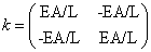
The linear bar element has only two degrees of freedom - one at each node. Consequently for a structure with n nodes, the global stiffness matrix is of size n × n (since there is one degree of freedom at each node).

Once the global stiffness matrix K is obtained, the structure equation is as follows:

{K}{U} = {F}

Where {U} the global nodal displacement is vector and {F} is the global nodal force vector. At this step the boundary conditions are applied manually to the vectors {U} and {F} . Then the matrix is solved by partitioning and Gaussian elimination. Finally, once the unknown displacements and reactions are found, the element forces are obtained for each element as follows:

{ f } = {k}{u}

Where { f } the 2 × 1 element is force vector and {u} is 2 × 1 element displacement vector. The element stresses are obtained by dividing the element forces by the cross-sectional area A.

Beam element: The beam element is a two-dimensional finite element where the local and global coordinates coincide. It is characterized by linear shape functions.

In the case of transverse loading, the beam element has modulus of elasticity E, moment of inertia I, and the length L. Each beam element has two nodes and is assumed to be horizontal as shown in Figure 2.

Figure 2: Beam Element.

In this case the element stiffness matrix is given by the following matrix, assuming axial deformation is neglected.

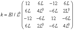
It is clear that the beam element has four degrees of freedom - two at each node (a transverse displacement and a rotation). The sign convention used is that the displacement is positive if it points upwards and the rotation is positive if it is counterclockwise. Consequently for a structure with n nodes, the global matrix K will be of size 2n × 2n (since we have two degree of freedom at each node).

Once the global stiffness matrix K is obtained, the structure equation is as follows:

{K}{U} = {F}

Where {U} is the global nodal displacement vector and {F} is the global nodal force vector. At this step the boundary conditions are applied manually to the vectors {U} and {F} . Then the matrix equation is solved by partitioning and Gaussian elimination. Finally, once the unknown displacements and the reactions are found, the nodal force vector is obtained for each element as follows:

{ f } = {k}{u}

Where { f } is the 4 × 1 nodal force vector in the element and {u} is the 4 × 1 element displacement vector. The first and second element in each vector {u} are the transverse displacement and rotation, respectively, at the first node, while the third and fourth element in each vector {u} are the transverse displacement and rotation, respectively, at the second node.

In the case of pure torsion, the beam element has modulus of rigidity G, polar moment of inertia J, and the length L. In this case the element stiffness matrix is given by the following matrix.

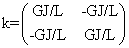
Here, the beam element has two degrees of freedom - one at each node (rotation). The sign convention used is that the rotation is positive if it is counterclockwise. Consequently for a structure with n nodes, the global stiffness matrix K will be of size n x n (since we have one degree of freedom at each node).

Once the global stiffness matrix K is obtained, the structure equation is as follows:

{K}{U} = {F}

Where {U} the global nodal displacement is vector and {F} is the global nodal torque vector. At this step the boundary conditions are applied manually to the vectors {U} and{F} . Then the matrix is solved by partitioning and Gaussian elimination. Finally once the unknown rotations and reactions are found, the element forces are obtained for each element as follows:

{ f } = {k}{u}

Where { f } the 2 × 1 element is torque vector and {u} is 2 × 1 element rotation vector. The element stresses are obtained by using the torsion equation as follows.

Where the element stress and r is the element radius (for circular cross-section).

As a result of the investigations focused on mechanical and thermal design parameters in the internal combustion engines, mechanical strength, thermal efficiency, wear and surface quality of the elements have been improved during the 20th century. Consequently, it can be clearly seen that fuel consumption has been reduced and engine lifetime has been increased. Erkaya et al. [10] Propose that In the case of conventional slider-crank mechanism, when piston is at top dead center, gas forces reach their maximum values. But any torque effect cannot be obtained for a small time interval due to this dead position, that is, torque output decreases. This situation does not occur in the modified mechanism with eccentric connector owing to structural arrangement. In the beginning of the power stroke, that is, when the driving force has its maximum value, force transmission is possible for both power transmission lines. Therefore, as opposed to conventional mechanism, torque output is directly proportional to driving force for the proposed mechanism. Daniel and Cavalca [11] Investigate the results indicated that the pin is subjected to two conditions during the operation. At some moments the pin is subjected to the hydrodynamic lubrication condition and at others it is in contact with the surface of the bearing. The numerical results indicated that the pin breaks the oil film, thus coming into contact with the surface of the bearing, regardless of the initial conditions or the parameters of the bearing. The solution of the problem of the slider-crank mechanism with hydrodynamic bearing in the connecting rod-slider joint is relatively complex due to the nonlinear equations of the models used in both hydrodynamic lubrication and the slider-crank mechanism. This set of equations presents high numerical stiffness, making the choice of the numerical integration method an important factor in the successful solution of differential equations. Wang and chen [12] Said that in industry, many applications of planar mechanisms such as slidercrank mechanisms have been found in thousands of devices. Typically due to the effect of inertia, these elastic links are subject to axial and transverse periodic forces. Vibrations of these mechanisms are the main source of noise and fatigue that lead to short useful life and failure. Hence, avoiding the occurrence of large amplitude vibration of such systems is of great importance. Vesa Saikko [13] Say the wear mechanisms were similar. Burnishing of the pin was the predominant feature. No overheating took place. With the dual motion HF-CTPOD method, the wear testing of UHMWPE as a bearing material in total hip arthroplasty can be substantially accelerated without concerns of the validity of the wear simulation. Reis et al. [14] Proposed that the research presents contribution in evaluating the effect introduced by hydrodynamic lubrication in the revolute joint clearance. Two models of hydrodynamic lubrication are investigated: the first model presents a direct solution of low computational cost, the second model results in a numerical solution that consider the effect of the acceleration of the lubricant fluid imposed on the movement of the mechanism. It was observed that the second lubrication model does not guarantee the support of the piston-pin system for hydrodynamic lubrication in the simulated interval of time. Therefore, it is necessary to develop a more realistic model of hydrodynamic and elasto-hydrodynamic lubrication that is capable of reproducing the behavior of the piston-pin contact.

The crankshaft, sometimes casually abbreviated to crank, is a large component with a complex geometry in the engine. It converts the reciprocating displacement of the piston to a rotary motion, or vice versa, with a four link mechanism. In addition, the linear displacement of an engine is not smooth, as the displacement is caused by the combustion of gas in the combustion chamber. Therefore, the displacement has sudden shocks and using this input for another device may cause damage to it. The concept of using crankshaft is to change these sudden displacements to a smooth rotary output, which is the input to many devices such as generators, pumps, and compressors (Figure 3).

Figure 3: Crankshaft.

The crankshaft consists of the shaft parts which revolve in the main bearings, the crankpins which are bearing surfaces whose axis is offset from that of the crankshaft, and the crank arms or webs which connect the crankpins and the shaft parts [8,15]. In a reciprocating piston engine, the crankpin serves the purpose of connecting the connecting rod to the crankshaft. It inserts into the big end of the connecting rod and is held by the big end cap. As the crankshaft experiences a large number of load cycles during its service life, fatigue performance and durability of this component has to be considered in the design process. Design developments have always been an important issue in the crankshaft production industry, in order to manufacture a less expensive component with the minimum weight possible and proper fatigue strength and other functional requirements. These improvements result in lighter and smaller engines with better fuel efficiency and higher power output [16,17].

Materials

The crankshaft is subjected to shock and fatigue loads. Thus material of the crankshaft should be tough and fatigue resistant. The crankshafts are generally made of carbon steel, special steel or special cast iron. In industrial engines, the crankshafts are commonly made from carbon steels such as 40C8, 55C8 and 60C4. In transport engines, manganese steel such as 20Mn2, 27Mn2 and 37Mn2 are generally used. In aero engines, nickel chromium steel such as 35Ni1Cr60 and 40Ni2Cr1Mo28 are extensively used for crankshafts.

Manufacturing

Crankshafts can be monolithic (made in a single piece) or assembled from several pieces. Monolithic crankshafts are most common, but some smaller and larger engines use assembled crankshafts. Crankshafts can be forged from a steel bar usually through roll forging or cast in ductile steel. Today more and more manufacturers tend to favour the use of forged crankshafts due to their lighter weight, more compact dimensions and better inherent dampening. With forged crankshafts, vanadium micro-alloyed steels are mostly used as these steels can be air cooled after reaching high strengths without additional heat treatment, with exception to the surface hardening of the bearing surfaces. The low alloy content also makes the material cheaper than high alloy steels. Carbon steels are also used, but these require additional heat treatment to reach the desired properties. Iron crankshafts are today mostly found in cheaper production engines where the loads are lower. Some engines also use cast iron crankshafts for low output versions while the more expensive high output version use forged steel. Crankshafts can also be machined out of a billet, often using a bar of high quality vacuum remelted steel. Even though the fibre flow (local inhomogeneities of the material’s chemical composition generated during casting) doesn’t follow the shape of the crankshaft (which is undesirable), this is usually not a problem since higher quality steels which normally are difficult to forge can be used. These crankshafts tend to be very expensive due to the large amount of material removal which needs to be done by using lathes and milling machines, the high material cost and the additional heat treatment required. However, since no expensive tooling is required, this production method allows small production runs of crankshafts to be made without high costs. Crankshafts can also be cast, but the above two methods are more popular. The surface of the crankpin is hardened by case carburizing, nitriding or induction hardening.

Stresses and failure in crankpin

The following two types of stresses are in the crankpin.

• Bending stress

• Shear stress due to torsional moment on the shaft

The crankpin is subjected to various forces but generally needs to be analysed in two positions. Firstly, failure may occur at the position of maximum bending (when the crank is at dead center). In such a condition the failure is due to bending and the pressure in the cylinder is maximum. Second, the crank may fail due to twisting, so the crankpin needs to be checked for shear at the position of maximum twisting. The pressure at this position is not the maximum pressure, but only a fraction of maximum pressure. The failure of a crankpin is likely to cause serious engine destruction.

Conventional design method

The crankpin is designed by considering two crank positions, i.e. when the crank is at dead center (or when the crankpin is subjected to maximum bending moment) and when the crank is at an angle at which the twisting moment is maximum. These two cases are discussed in detail as follows.

When the crank is at dead center: At this position of the crank, the maximum gas pressure on the piston transmits maximum force on the crankpin in the plane of the crank causing only bending. The crankpin is only subjected to bending moment. Thus, when the crank is at dead center the bending moment on the shaft is maximum and the twisting moment is zero

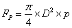
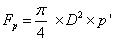
The gas load on the piston,

Where,

D= Piston diameter in mm

p=Maximum intensity of pressure on piston in N/mm² Now consider a single throw crankshaft as show in Figure 4.

Figure 4: Crank at Dead Centre.

Due to the piston gas load acting horizontally, there are two horizontal reactions and at the bearings 1 and 2 respectively.

Let, d_c = Diameter of the crankpin in mm

l_c = Length of crankpin in mm

σ_b =Allowable bending stress for the crankpin in N/mm²

Now, bending moment at the center of crankpin,

We also know that,

From the above relation, diameter of the crankpin is determined.

The length of the crankpin is given by,

Where, p_b =Permissible bearing pressure in N/mm²

When the crank is at an angle of maximum twisting moment: The twisting moment on the crankshaft is maximum when the tangential force on the crank (FT) is maximum. The maximum value of the tangential force lies when the crank is at an angle of 25° to 30° from the dead center for petrol engines and 30° to 40° for diesel engines.

Consider the position of the crank at maximum twisting moment shown in Figure 5.

Figure 5: Crank at Position of Maximum Twisting Moment.

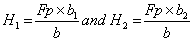
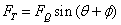
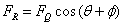
Let be the intensity of pressure on the piston at this instant, then the piston gas load at this position is given by:

Thrust on the connecting rod is:

Tangential force (cause of twisting) on the crankpin is:

Radial force (cause of bending) on the crankpin is:

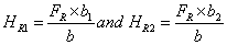
Due to tangential force F_T there will be two reactions on bearing 1 and 2:

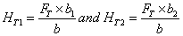
Due to radial force FR there will be two reactions at bearing 1 and 2:

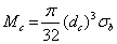
Now, bending moment at the center of crankpin,

And twisting moment on the crankpin,

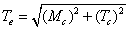
Therefore, equivalent twisting moment in the crankpin,

The diameter of the crank pin can be calculated using the following relation:

Where τ = Allowable shear stress in the crankpin.

While designing the crankpin, the following dimensions are required to be determined:

• Length of crankpin.

• Diameter of crankpin (larger value of above two cases is taken).

The MATLAB program developed for conventional design of crankpin. A crankpin for the following data is designed using the MATLAB program.

Speed of engine=200 rpm Bore=400 mm

Crank radius=300 mm

Ratio of connecting rod length to crank radius=5

Distance between bearings and center of crankpin=400 mm

Maximum combustion pressure=2.5 N/mm²

Crank angle at position of maximum twisting moment=35°

Cylinder pressure at position of maximum twisting moment=1 N/ mm²

Allowable bending stress for crankpin=75 N/mm²

Allowable shear stress for crankpin=35 N/mm²

Modulus of elasticity=207000 N/mm²

Modulus of rigidity=82000 N/mm²

The following solution is obtained (values are rounded-off):

Diameter of crankpin=204.35 mm (205 mm)

Length of crankpin=153.7 mm (154 mm)

The above dimensions (rounded-off values) are used for FEA of the crankpin in the following section.

Finite element analysis of crankpin

(A) Load analysis: When the crank is at dead center, the maximum gas load on the piston is transmitted to the crankpin and is assumed to act as uniformly distributed load acting along the length of the crankpin.

The gas load on the piston obtained during conventional design is 314.2 kN.

When the crank is at the angle of maximum twisting moment, the equivalent twisting moment due to the bending and twisting loads is assumed to act at the center of the crankpin.

The equivalent twisting moment acting at the center of crankpin obtained during conventional design is 22.8×10⁶ N-mm.

(B) Boundary conditions: The crankpin is assumed to be acting as a fixed-fixed beam under all conditions.

When at the dead center, it is assumed that a uniformly distributed load is acting on all the nodes except the end nodes which are fixed (Figure 6).

Figure 6: Crankpin at dead center.

When at the position of maximum twisting moment, it is assumed that the equivalent twisting moment is acting on the central node and the end nodes are fixed (Figure 7).

Figure 7: Crankpin at angle of maximum twist.

(C) Finite element analysis: The conventional deign method gives the geometry of the crankpin, and the load conditions are obtained after load analysis. These results are finally used to carry out the finite element analysis of the crankpin on the basis of the assumed boundary conditions.

First, the analysis is carried out at the dead center. The crankpin is discretised using beam elements. A MATLAB program is developed for this purpose.

Using 35 and 355 elements, the following two plots (on next page) for shear stress distribution along the length of the crankpin are obtained.

It can be seen from the plots that the maximum stress in the crankpin is about 4.8 N/mm² which is appreciably lower than the allowable shear stress (35 N/mm²), indicating that the design is safe (Figures 8 and 9).

Figure 8: Crankpin stress distribution.

Figure 9: Crankpin stress distribution.

Next, the analysis is carried out at the position of maximum twisting moment. The crankpin is discretised using beam elements (torsional). A MATLAB program is developed for this purpose.

Using 100 elements, the following plot (on next page) for shear stress distribution along the length of the crankpin is obtained. It can be seen from the plot that the maximum shear stress in the crankpin is about 6.8 N/mm², which is appreciably lower than the allowable shear stress, indicating that the design is safe.

Higher number of elements can be used, but no increase in accuracy will be seen as the stress distribution is uniform (Figure 10). This concludes the chapter on Crankpin

Figure 10: Crankpin stress distribution.

This study has helped in carrying out performance analysis of critical components of an internal combustion engine. Detailed stress/strain distributions have been obtained as a result of analysis of crankpin by using the finite element method. The results have been compared with the conventional design of each component to judge whether the design is safe or not. Thus, the analysis acts as a measure of the components safety and reliability. The MATLAB programs that have been developed for this purpose can be used to analyse any design under various load conditions. The stress/strain distributions help in identifying areas that have high stress concentrations as well as areas that have high factor of safety due to presence of excess material. This can help the designer in optimization of the components by altering the designs according to the computed stress distributions. Due to its large volume production, it is only logical that analysis for optimization of the engine components will result in large-scale savings. It can also achieve the objective of reducing the weight of the engine components, thus reducing inertia loads, reducing engine weight and improving engine performance and fuel economy. Dual goals of cost reduction and efficiency can be achieved simultaneously. The apparent strength and precision of the finite element method portray it as a powerful tool for engineering analysis. It also serves as a basis of comparison of different designs. This study encompasses two-dimensional static stress analysis. The work carried out in this study can be improved upon by including dynamic effects and using three-dimensional approach to get more accurate results.