Journal of Geology & Geophysics
Open Access
ISSN: 2381-8719
ISSN: 2381-8719
Research Article - (2015) Volume 4, Issue 6
The quantitative results obtained from the use of spectral analysis technique, Source parameter Imaging technique and empirical depth rule method (maximum and half slope techniques) in interpreting High Resolution AeroMagnetic of middle Benue trough data have been presented and compared. Before employing each technique, the regional residual seperation was done with least square method using polifit program to get the residual data for onward processing. The slope technique usually require that the residual values be contoured into map and then profiled along the most prominent anomaly to obtain the depth curves from where depth to magnetic sources could be calculated. The Spectral requires that the residual values be sub-divided into spectral blocks and radial energy spectrum be generated from where depth would be calculated from the slopes of the straight line plots. The SPI requires the griding of the residual values and the conversion of this to image map from where depth could be read off easily. The deep magnetic anomally source gotten ranges from 2.00 km to 6.29 km with an average depth of 3.25 km for SPI technique; 2.33 km to less than 5.66 km with an average depth of 3.65 km for Spectral analysis technique; and average of 3.74 km and 3.66 km for Half-slope and maximum slope technique respectively. These average depth could be taken as the magnetic basement depth and has the significant that if other conditions are met, this study area of marine sedimentary layer of the Albian Age is favourable for hydrocation accumulation. The shallow source depth gotten ranges from 0.02 km to 2.00 km with an average depth of 1.08 km for SPI; 0.05 km to less than 0.42 km with an average depth of 0.21 km for spectral analysis; and an average depth 0.80 km for Half slope technique. This can be viewed as magmatic intrussion into the sediment and could be responsible for the lead-Zinc mineralization found in the area. These methods thus compares favourably well and moreso the slope technique though empirical has compared favourably with more modern automatic source depth methods.
Keywords: High resolutio aeromagnetic data(HRAM), Magnetic anomaly; Spectral analysis, Source parameter imaging, Slope techniques, Magnetic basement depth
Aeromagnetic Data analysis is an important tool in maping the magnetic basement depth beneath the sedimentary cover. One of the important parameter in quantitative interpretation is the depth of the anomalous body. In oil exploration, basement depth is needed which we have obtained through the empirical method based on slope technique (maximum and half-slope), the Spectral technique, and source parameter imaging techniques (SPI) [1-3]. This work seeks to compare these methods and their results.
The spectral analysis and SPI technique used here are amongst the modern automatic source depth method of determining magnetic basement depth. The slope techniques (the maximum and half slope technique) is an empirical methods based on slope techniques using empirical constants. This work has employed these methods to quantitatively interprete the HRAM data obtained from the most recent survey in the country. This work seeks to obtain the magnetic basement depth of the studied area, the basement topography and contour orientations and appraise the hydrocarbon accumulation potential of this area. It also looked at the advantages of these methods over one another and how they compared amongst themselves and those of other researchers.
Geography of the study area
The aeromagnetic map of Nigeria is shown in Figure 1a. The geographical cordinates of the study area is between Latitude 7.00’N to 8.00’N and Longitude 8.50’E to 9.50’E. It is represented by sheet numbers 251, 252, 271, 272 shown by Figure 1b.
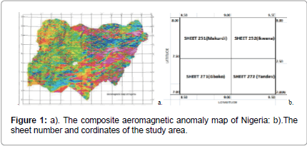
Figure 1: a). The composite aeromagnetic anomaly map of Nigeria: b).The sheet number and cordinates of the study area.
Each square block of Figure 1b represents a map on the scale of 1:100,000. Each square block is (55 × 55) km2 covering an area of 3,025 km2, hence the study area is 12,100 km2.
The geology of the study area
The study area (the hatched portion in Figure 1c) is located in the middle Benue trough sedimentary basin Nigeria. Nigeria is made up of about seven inland sedimentary basins which are shown in Figure 1c. The Benue Trough is divisible into upper, middle and lower Benue trough. It originated from the early Cretaceous rifling of the Central West African basement uplift.
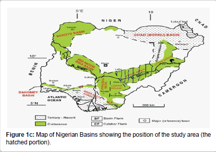
Figure 1c: Map of Nigerian Basins showing the position of the study area (the hatched portion).
As shown in Figure 1d, the study area is characterized by the presence of thick sedimentary cover of varied composition whose age ranges from Albian to Maastrichtian, with the earliest sedimentation being the marine Asu-River group of Abian age [4].
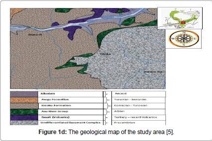
Figure 1d: The geological map of the study area [5].
Stratigraphically, the Cretaceous sedimentary succession in the study area as shown on Figure 1d,e comprise of the Asu -River Group of marine origin which is the oldest deposited sediment in the Middle Benue Trough followed by Ezeaku Formation, keana/Awe Formation, Awgu Formation and Lafia Sandstone as the youngest sediment [5]. The works of [6-10] have more on the geology of the Benue Trough. The important of the knowledge of the geology of the study area is with regards to hydrocarbon formation, as oil are usually formed from the remains of dead marine animals. The studied geology have therefore revealed that the earliest sediment in the study area is oil accumulation favourable Asu-river group of marine origin as obtainable in oil rich Niger-Delta part of the country.
The aeromagnetic map of the digitized HRAM data used for this work is shown on Figure 2a. It was purchased from the Nigerian Geological Survey agency Abuja Nigeria, from the most recent 2009 survey caried out by Fugro Airborne service. This data is in digitized form eliminating possible errors usually introduced during digitization of the old 1970’s map. It is of higher resolution than those of 1970’s which are in map form being flown at 500 m line spacing and 80 m terrain clearance as against the 1970’s flown at a flight line spacing of 2 km, average terrain clearance of 150 m, and a nominal tie line spacing of 20 km. The HRAM data of the four different blocks was assembled and imported into SUFER32 software and used to produced the composite anomaly map of Figure 2b.
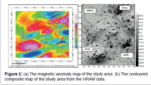
Figure 2: (a) The magnetic anomaly map of the stydy area. (b) The contoured composite map of the study area from the HRAM data.
Amongst the notable researchers who have worked in this area with the old data of 1970’s include [11-13].
Reduction to the pole
The aim of reduction to pole is to produce magnetic map that would represent an area being surveyed at the magnetic pole from the observed total magnetic field map. Assuming that all the observed magnetic field of the study area is due to induced magnetic effects, pole reduction can be calculated in the frequency domain using the following operator [14].
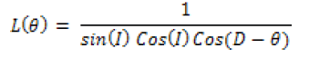
Where
In reduction to the pole procedure, the measured total field anomaly is transformed into the vertical component of the field caused by the same source distribution magnetized in the vertical direction. The acquired anomaly is therefore the one that would be measured at the North magnetic pole, where induced magnetization and ambient field both are directed downwards [15].
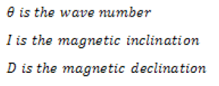
For potential field data like magnetic and gravity to be interpreted, the residual anomaly must be separated from the regional background field. Usually the targets are the anomalies of the basement rock, and their magnetic field is superimposed in the regional field that comes from larger deeper sources and the magnetic effect of all the underground magnetic sources. The regional field was modeled with a first order polynomial and the residual field regarded as an error between the model and the data using Polifit program. The residual data obtained was contoured into 2-D and 3-D maps in Figure 3a,b giving us the first impression of the study area.
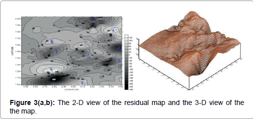
Figure 3(a,b): The 2-D view of the residual map and the 3-D view of the the map.
The major anomalies in the 2-D contour map have been numbered 1-10 and these are the magnetic signatures of the subsurface basement rocks. The anomalies are divisible into low frequency anomalies (1,3,4,7,9,10) coming from deep seated bodies and high frequency anomalies (2,5,6,8 )from shallow seated bodies. Juxtaposing the 2-D and 3-D maps revealed more clearely the undulations and likely traps in the basement surface. The orientation of the magnetic contours could be observed to be predominantly in NE-SW direction with subordinate E-W direction. Markudi area is more featureless while Gboko has interesting geological features and should be the exploration targets in the studied area.
The theory and the result of the slope method, spectral analysis and the SPI used have been presented here.
The slope technique (maximum and half-slope): [16] was probably the first to relate depth of magnetic source to the horizontal extent of the portion of sloping flanks of his profile curves as illustrated in Figure 4.
Figure 4: Determining anomaly depth from the slope of magnetic profile. Maximum slope(S); Peters Half-slope (P) [17-19].
Usually to estimate magnetic depth from this method, the horizontal extent of the portion of the profile curve that is nearly linear at the maximum slope (S) is measured, or the distance between the two points of tangency (half slope, {P} ) is measured. The depth (Z) beneath the portion of the curve is calculated using equation 1.0 and 2.0 [17-19].
Z= K1S ; 1.67 ≤ K1 ≤ 1.82 (empirical constant K1 1.82)……………1.0
Z = K2P (empirical constant K2 = 0.63) ………..2.0
To generate curves and calculate magnetic source depth, the residual contour map of Figure 3a was profiled NNI, BBI, AAI, OOI and WWI along the most prominent anomaly zones within the study area as shown on the profile map of Figure 5a [2].
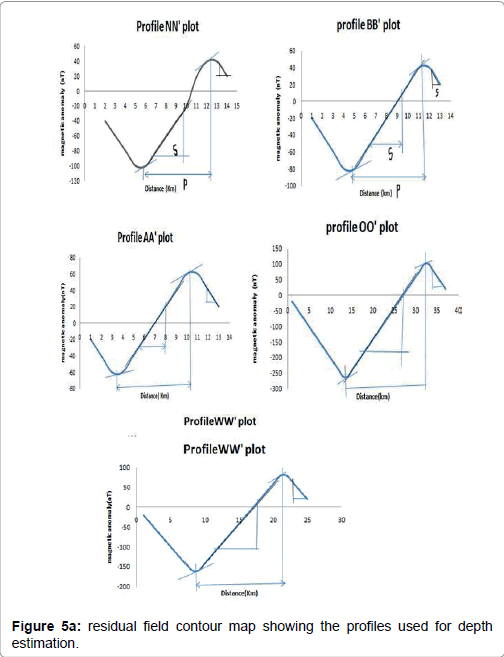
Figure 5a: residual field contour map showing the profiles used for depth estimation.
The ploted magnetic profile curves which is a replica of the theoretical curves have been presented in Figure 5b.
Employing the theoretical equations of 1.0 and 2.0, the summary of the estimated depths for the five profiles taken are shown on Table1 using the maximum and half slope techniques.
| PROFILES | MAXIMUM SLOPE TECHNIQUE (for the deep and shallow source) | HALF SLOPE TECHNIQUE (deep source) | ||||||
| DEEP | SHALLOW | Depth (Z)=K1P | Depth (Z)=K2P | |||||
| S (km) | S (km) | Constant (K1) | Deep (km) | Shallow (km) | Deep (km) | Constant (K2) | Depth (km) | |
| NN' | 2.0 | 0.3 | 1.82 | 3.64 | 0.36 | 6.6 | 0.63 | 4.16 |
| BB' | 2.0 | 0.3 | 1.82 | 3.64 | 0.36 | 6.6 | 0.63 | 4.16 |
| AA' | 1.8 | 0.8 | 1.82 | 3.23 | 1.46 | 5.2 | 0.63 | 3.28 |
| OO' | 2.4 | 0.5 | 1.82 | 4.36 | 0.91 | 6.8 | 0.63 | 4.28 |
| WW' | 1.9 | 0.5 | 1.82 | 3.45 | 0.91 | 4.5 | 0.63 | 2.83 |
| Average depth from each slope technique | 3.66 | 0.80 | 3.74 | |||||
| Estimated magnetic basement depth from the slope method=3.70 km | ||||||||
Table 1: Summary of depth estimate from the slope techniques.
The average magnetic basement depth from these two method is 3.70 km. It is important to use both the maximum and half slope method for they provides a check on the depth estimate and the care with which the graphical analysis is done.
The spectral technique: The application of the power spectrum method to potential field data has been well establised, and the determination of the anomalous body depth has also been given [20,21]. This method has been used extensively by many researchers like [22,23].
In its complex form, the two dimensional Fourier transform pair may be written as in eqn 3.0 and 4.0 [20,24]:
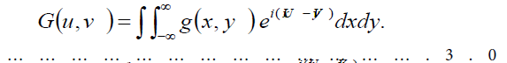 … … … … … … … … … … … … … . 3.0
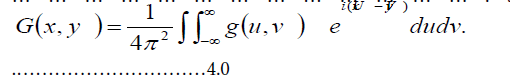 .…………………………4.0
Where u and v are the angular frequencies in x and y directions respectively
For depth estimations for magnetic field data this was expressed as
E(u,v)=exp(-2hr) [21] ………………………………………………………………….5.0
The exp (-2hr) term is the dominant factor in the power spectrum. The average spectrum of the partial waves falling within this frequency range is calculated and the resulting values together constitute the redial spectrum of the anomalous field. If we replace h with Z and r with f; then
Log E = -2Zf ……………………………………………………..6.0
Where Z is the required anomalous depth; and f frequency. Therefore the linear graph of logE against f leaves slope (m) =-2Z. The mean depth (Z) of the magnetic source is thus given by
Z=m/2. ………………………………………………...7.0
Employing this technique involves
-Divisions into Spectral cells and Windowing: The four residual blocks of the study area was subdivided into 16 spectral cells of 12.5 km by 12.5 km for easy handling of the large data involved and each signal was widowed 15 minutes by 15 minutes.
-Generation of radial energy spectrum: Digital signal processing software the Oasis Montaj was used to transform the residual magnetic data into the radial energy spectrum for each block.
-Plots of Log of Energy and the frequency: [21] have shown that the Log-power spectrum of the source has a linear gradient whose magnitude is dependent upon the depth of the source. The spectral energy against frequencies for the 16 spectral cells was plotted and shown on Figure 6.
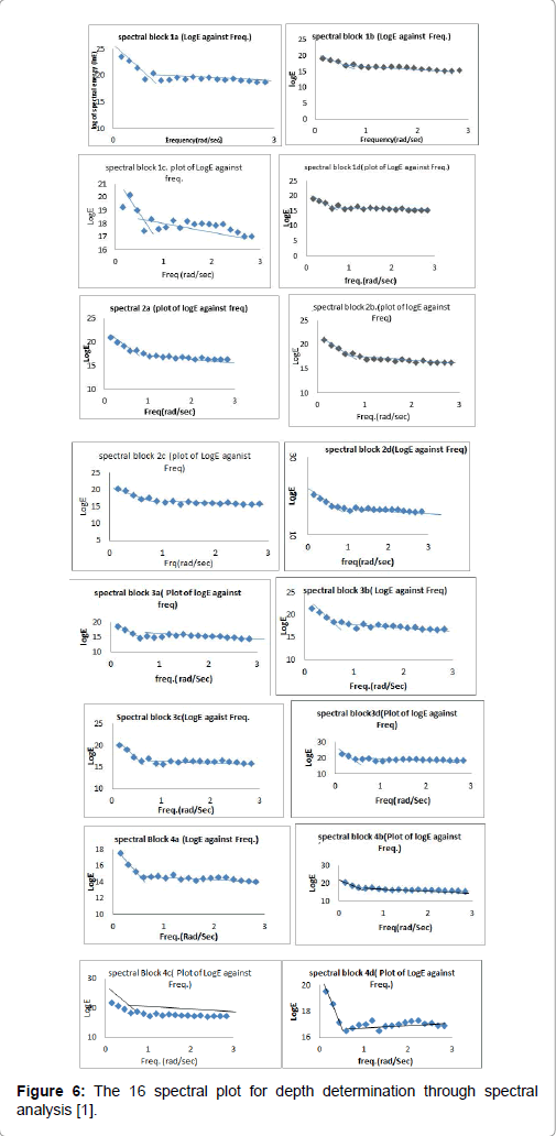
Figure 6: residual field contour map showing the profiles used for depth estimation.
These series of points which fall on one or more straight line segments represent bodies occurring within a particular depth range. The line segment in the higher frequency range is from the shallow sources and the lower harmonics are indicative of sources from deep seated bodies.The slope of these provide a measure of the mean depth to the ensemble of the anomalous bodies.
- Estimation of the depth to magnetic sources: The gradients  of each of the line segments were first evaluated. The mean depth (z) of burial of the ensemble given as
  was then calculated [21]. The coordinates and the two depth estimates (z1 and z2) for each of the sixteen spectral blocks are given on Table 2.
| S/No | SPECTRAL BLOCKS | CO-ORDINATES | SLOPES (M) | DEPTH (M/-2) | |||
| SECTIONS | X (Longitude) | Y (Latitude) | DEEP (m1) | SHALLOW (m2) | DEEP (Z1) | SHALLOW (Z2) | |
| 1 | 1A | 8.63 | 7.12 | -11.32 | -0.42 | 5.66 | 0.21 |
| 2 | 1B | 8.63 | 7.37 | -6.07 | -0.84 | 3.04 | 0.42 |
| 3 | 1C | 8.63 | 7.62 | -4.46 | -0.40 | 2.23 | 0.20 |
| 4 | 1D | 8.63 | 7.88 | -6.86 | -0.53 | 3.43 | 0.27 |
| 5 | 2A | 8.88 | 7.13 | -6.31 | -0.44 | 3.16 | 0.22 |
| 6 | 2B | 8.88 | 7.38 | -6.31 | -0.44 | 3.16 | 0.22 |
| 7 | 2C | 8.88 | 7.63 | -7.97 | -0.57 | 3.98 | 0.28 |
| 8 | 2D | 8.88 | 7.88 | -6.35 | -0.45 | 3.17 | 0.22 |
| 9 | 3A | 9.13 | 7.13 | -7.42 | -0.24 | 3.71 | 0.12 |
| 10 | 3B | 9.13 | 7.38 | -6.86 | -0.62 | 3.43 | 0.31 |
| 11 | 3C | 9.13 | 7.63 | -8.73 | -0.18 | 4.37 | 0.09 |
| 12 | 3D | 9.13 | 7.9 | -7.88 | -0.15 | 3.94 | 0.07 |
| 13 | 4A | 9.38 | 7.13 | -6.6 | -0.26 | 3.30 | 0.13 |
| 14 | 4B | 9.38 | 7.38 | -8.89 | -0.66 | 4.44 | 0.33 |
| 15 | 4C | 9.38 | 7.63 | -7.82 | -0.54 | 3.91 | 0.27 |
| 16 | 4D | 9.38 | 7.88 | -6.99 | 0.09 | 3.50 | 0.05 |
| AVERAGE DEPTH | 3.65 km | 0.21 km |
Table 2: depth estimates of the first and second magnetic layers for the 16 spectral blocks and their coordinates.
Therefore the result of the spectral analysis of aeromagnetic data over the project area suggests the existence of two main source depths; the deeper sources (z1) (2.23 km- 5.66 km; and avg of 3.53 km) represented by the steeper line of figure 6 and the shallow sources (z2) (0.05 km -0.42 km, avg of 0.21 km) represented by the other line.
Source parameter imagin (SPITH )
The SPITH method based on [25] method utilizes the relationship between source depth and the local wavenumber (k) of the analytic signal of the observed field. This can be calculated for any point within a grid of data via horizontal and vertical gradients to estimated magnetic depth.
The analytic signal A1(x,z) is defined by [26] as
 ……………………………………………………………………..5.0
Where M(x,z) is the magnitude of the anomalous total magnetic field, j is the imaginary number, and z and x are Cartesian coordinate for the vertical direction and the horizontal direction perpendicular to strike, respectively. The local wave number K1 and K2 is expressed as.
 ……………………………………………………………………..6.0
 ………………………………………………………………….….7.0
Where nk is the SPI structural index (subscript k=c, t or h ), and nc=1 and nh=2 for the contact, thin sheet and horizontal cylinder models and hk is the depth to the top of the contact, respectively. The result of this analysis is displayed on an image and the correct depth estimate for each anomaly can also be determined. OASIS MONTAJ software was employed to grid the data and compute the SPI image and depth. SPI method makes the task of interpreting magnetic data significantly easier as shown by the SP images generated from residual field data of the studied area on Figure 7 [3].
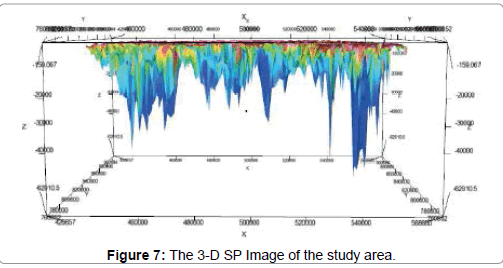
Figure 7: The 3-D SP Image of the study area.
The ends of the peak could be traced to the depth axis (Z) and the values read. The longest spikes are blue showing deep lying bodies and the shortes spikes are orange and pink showing shallow seated bodies. The depth values obtained from this method is displayed on Table 3.
| SPI obtained depth | Range | Average Depth (km) |
| Deep lying magnetic bodies | 2.00 km - 6.29 km | 3.25 km |
| represented by long blue spikes | ||
| Shallow lying magnetic bodies | 1.59 km - 2.00 km | 1.08 km |
| represented by short spikes |
Table 3: Depth values from the image of Figure 7.
| Quantitative techniques employed | Avg estimated magnetic basement depth | Avg estimated shallow magnetic sources depth |
| SLOPE techniques | 3.70 km | 0.80 km |
| Spectral technique | 3.65 km | 0.21 km |
| Spi technique | 3.25 km | 1.08 km |
Table 4: Deep and shallow source depth from Slope, Spectral and SPI techniques.
The preliminary qualitative interpretation of the aeromagnetic data of part of middle Benue trough Nigeria described above have revealed two magnetic anomaly sources; the low frequency anomaly source related to deep seated bodies and the the high frequency anomaly source related to shalow seated magnetic bodies. The areas of deep seated bodies in the map are possibly the magnetic basement depth; while the shallower are possibly magmatic/igneous intrusions into the sedimentary basins which are possibly responsible for the leadzinc mineralization found in the area. This findings is in conformity with those of previous researchers which used the 1970’s old data. This qualitative interpretations of the residual map also revealed conjugate pair of NE-SW and NW-SE fracture in the Benue trough as have been predicted earlier by the works of [27] which was attributed to the event at possible opening up of African and South American plates. Several undulations and likely traps have equally been found on the basement surface which could likely form traps for hydrocarbon accumulation. The spectral analysis and Landsat Imagery of the adjacent lower Benue trough by [28] equally revealed a two layer depth model and predominant NE-SW lineament trend.
The results of the quantitative interpretation to determine the deep and shallow magnetic sources using Slope, spectral and SPI technique have been presented on Table 3.
The revelation from the spectral study of 3.65 km, Slope techniqe study of 3.70 km and SPI study of 3.25 km respectively represents the magnetic basement depth. These are synonymous to depth of over-burden sediment in the study area which has a very important significance as regards to the hydrocarbon generation potential of the area. Previous study showed the geology of the area to be associated with the marine Albian Asu River Group which commenced sedimentation in the middle Benue Trough.
A researcher [29] has pointed out in his work that if all other conditions for hydrocarbon accumulation are favourable, and the average temperature gradient of 1°C for 30 m obtainable in oil rich Niger Delta of the country is applicable, then the minimum thickness of the sediment to achieve the threshold frequency temperature of 115°C for the commencement of oil formation from marine organic remains would be 2.3 km depth. Thus on the basis of the average estimated magnetic basement depth of the study area from Table 3, and the probable marine source bed of Asu River group in the lower/ middle sector of the Nigerian Benue trough and the likely traps found in the basement surface of the study area, the area could be looked upon as favourable and very promising for hydrocarbon accumulation especially the Gboko axis. The shalow magnetic source depth from Table 3 is probably magmatic intrussion into the sediment and this could be responsible for the Lead-Zinc mineralization found in the study area. Active magmatism have been reported in the Benue trough and the work [30] have confirmed the close association between magmatism, mineralization and fractures in the Benue Trough.
These three independent techniques gave depth values that are similar to each other and comparable to those obtained by previous researchers who employed the old data.
The spectral analysis and Landsat Imagery of the adjacent lower Benue trough by [28] revealed an average depth of 3.574 km for the deeper magnetic source bodies, and average shallower magnetic source depth of 1.041 km. [11] estimated the magnetic basement depth of the middle Benue Trough to be between 2.00 km - 4.00 km, considering it to be the most prospective area within the trough. Depth to the magnetic basement from the spectral work of [13] vary from 1.513 km and 4.936 km. The gravity work of [10] over the upper Benue Trough estimated the thickness of the sediments between 0.9 km and 4.6 km.
Discusions and comparisons of the analysis techniques
Although the slope method is an old pre-computer method based on empirical constant developed out of enormous experience in magnetic interpretation acquired over the years, but it has given result that is comparable to the more modern automatic source depth method of Spectral and SPI. It’s a graphical techniques which make use of the sloping flanks of profile to estimate depth. The slope techniques generally yields reasonable result for horizontal basement models with steeply dipping contact. It is much simpler and faster and provides more depth estimate than analysis by model curve fitting. This method is mostly used as a quick check on the validity of depth estimates.
A serious advantage of SPI over spectral analysis as automatic source depth techniques is that SPI is a profile or grid-based method for estimating magnetic source depths and does not require a moving window.In Spetral analysis, for small windows of data the limited number of grid nodes often leads to power spectra becoming jagged at the start or end. This is the reason for omitting the first point in the automated determination of the deepest straight-line segment of the power spectra. SPI method makes the task of interpreting magnetic data significantly easier as depth can be displayed as an image as earlier shown (Figure 7). The depth estimate can be summarized on one map independent of an assumed model which can be interpreted even by non-expert in the field, and the computation time is relatively short. However, the interpretation of the gravity and magnetic data is preferred in frequency domain because of simple relations between various source models and field [31]. The power spectrum of the surface field can be used to identify average depths of source ensembles [21]. The technique of spectral analysis provide rapid depth estimates from regularly- spaced digital field data, no geomagnetic or diurnal correction are necessary here as these remove only low wave number component and do not affect depth estimate which are controlled by high wave number component of the observed field [32]. The output of this operation is the radial spectral energy and frequency. These can be plotted in straight line graphs and further analysis like gradients calculation done before depth could be calculated from these gradients as already shown.
The preliminary qualitative interpretation of the anomalies in the 3-D and 2-D residual map revealed areas of high frequency anomaly sources related to deep seated bodies and areas of low frequency anomaly related to shallow seated bodies. Several undulation and likely traps is noticeable on the basement surface. Predominant NESW with surbodinate E-W contour trendings, an attribute of the Pan–African Orogeny trends was equally found. SPI, spectral and slope techiques was now used to quantitatively determine the depth of the deep and shallow seated bodies. The magnetic basement depth values from these techniques compares favourably with themselves and that of other researchers who used the old 1970’s map. The study area has been confirmed to be favourable for oil accumulation if other conditions are met especially the Gboko area with good geological features and likely traps. However, these magnetic basement depth gotten using the the high resolution 2009 data is more solid than that gotten using the 1970’s data.This is because of the improved flight parameters, imporovement in technology and various error correcting softwares used during the acquisition of the digitized 2009 data.