Journal of Geology & Geophysics
Open Access
ISSN: 2381-8719
ISSN: 2381-8719
Research Article - (2023)Volume 12, Issue 5
Subsidence of the Earth’s crust has allowed sediments to accumulate on the top of a basement of igneous and metamorphic rocks in form of sedimentary basin. These sediments and associated fluids are chemically and mechanically transformed through the several physical events like compaction and heating to a course of time. Consequently, it becomes the reservoir of the energy resources of petroleum, natural gas, coal, geothermal energy, and uranium etc. Their generation, development and disappearance are directly related to plate tectonic movements and other important geological events to understand the evolution history. Therefore, it is very crucial to evaluate the thickness of the sediments in terms of basement relief to highlight the depositional settings and basin formation factors. Here, we have developed a MATLAB based Artificial Neural Network approach to obtain the depth of a sedimentary basin considering the density variation with depth. In this work, a synthetic model is created initially by using 2D rectangular prism and later the model is perturbed with a 5% Gaussian White Noise. A supervised learning process is used to train the neural network and backpropagation with stochastic gradient descent technique is used to optimize the network output. The prism model is then used to create synthetic sedimentary basin to determine the depth profile with known density contrast using computed gravity datasets. After checking this optimization for various synthetic model, the technique is used on real data taken from Sayula Basin, Mexico and the results are compared with previous basement depths to validate its efficacy. The novelty of the proposed neural network approach is fast and efficient computation without any initial model assumptions that can map complex input output relations very efficiently, where other optimization process lack in this segment.
Sayula Basin; Deep Neural Network (DNN); Sedimentary; Gravity data
The formation of sedimentary basin and its sequential depositional history in a subsidence environment are conspicuous phenomenon in geological field. Such type of geological formation provides most geological resources and raw materials to mankind such as oil, gas, coal, drinking water, geothermal water, building materials and lead to the precipitation of a wide range of ore deposits [1-3]. These deposits in form of sedimentary layers hold the records of the past geological history and crustal variation including tectonic events, climatic condition, changes in sea level, morphological changes, earthquake history, migration history of living creatures, and other environmental modifications [4,5]. However, the most essential element of the formation is tectonic creation of basement relief to provide both a source of sediments and a relatively low place for the deposition of that sediment to experience a variety of transformation [6,7]. Therefore, sedimentary basins are playing a pivotal role in geological evolutionary through vast research on the deposition of sediment types, sediment thicknesses in terms of basement relief, and paleo-currents in a basin that offer evidence of the existence and location of elevated areas of the crust created by tectonism [8,9]. Hence, there is an ironic tradeoff between having more complete preservation in the subsurface but less satisfactory observations due to exposed basins at the surface are undergoing destruction and loss of record by erosion. In contrast, delineating the basement relief directly suggest the referred depth as the tectonic subsidence and uplift of the regions to conclude the types of sedimentary basin [10]. Concurrently, it is not so obvious to estimate the basement relief of the sedimentary basin using geophysical data due to the different stages of loading, thermal contractions, orogenic loading, compaction, paleo-environment and sea level changes that all contribute towards the heterogeneous variations in density. Since the early 80s several attempts were continuously made to construct the basement relief of sedimentary basin using geophysical data majorly from gravity anomaly using constant density throughout the basin and subsequent models considered more realistic schemes for the basement estimation followed by updated optimization schemes from classical to recent advanced optimization tools.
Gravity data leads to properly image the subsurface structure or the causative bodies although having inherent ambiguity in them and therefore results to non-unique solution when they are inverted. It also offers ill posed solution and erroneous in nature where is no unique solution. Any priori information about the causative body can help to eliminate the problem of gravity inversion. Implementation of constraints [11,12], and introducing proper regularization [13], can help to get a stable solution over noisy data also. Proper uncertainty appraisal also helps to overcome the non-uniqueness of the inverse problem [14,15], while determining the model parameters. Interpretation of gravity data by inversion technique leads to position and depth and density estimation of the causative body [16]. Computational development toward the basement relief of sedimentary basin has significantly improved in mineral exploration [17,18], hydrocarbon exploration [19], fault structure analysis [20,21], hydrology [22], glaciology [23], CO2 sequestration [24], etc. In a gravity inversion problem of sedimentary basin, there is two vital unknown parameters like density variation and geometry of the source respectively. Any prior knowledge about one of them can reduce the dimension of the parameter space as a constraint and provides a unique solution. So, the depth of any sedimentary basin can be obtained using any prior knowledge of physical parameter. Most of the cases density is used as the known parameter, which may be constant throughout the structure [25,26], or it may have a vertical variation. In real cases of basin formation, density is not constant but changes throughout the vertical lateral extent, which may be linear or nonlinear [8,27,28]. Now using any optimization technique will lead to estimation of unknown parameter. Generally, density value is estimated from borehole or well log data. From these datasets density as a function of depth can be calculated mathematically. Many scientists worked on the modelling of 2D sedimentary basin with vertically varying density contrast and calculated the depth of those basins. Radhakrishna et al. [29], and Chappell et al. [30], used an exponential density distribution. Hansen et al. [31], introduced linear density-depth relationships, Litinsky et al. [32], and Sari et al. [33], took a hyperbolic density function, Martin-Atienza et al. [34], calculate second-order polynomial functions of density contrast for sedimentary basin.
In earlier decades, few researchers had attempted to estimate the basement depth using classical inversion scheme like Fourier transformation [35], Euler deconvolution [36], Mellin transform [37], Hilbert transform [38], Hartley transform [39], least-squares minimization [40], and Walsh transform [41], and therein. Recently, gravity inversion for the basement relief estimation was also done with some scattered knowledge of the basement depth from boreholes even without any prior knowledge of density value [42]. Kaftan et al. [43], used genetic algorithm to determine the depth of buried structures. Particle swarm optimization technique is also used to invert the potential field data [17,44-48]. Levenberg–Marquardt algorithm is used for gravity inversion by Chakravarthi et al. [20], a nonlinear conjugate gradient for combined gravity and gravity gradient inversion [49], Florio et al. [50], used iterative rescaling to estimate the depth to the basement in a 3D scenario [51,52]. Feng et al. [53], used combined multinorm and normalized vertical derivatives with nonlinear conjugate gradient for 3D gravity inversion of basement relief. Silva et al. [54], used a fast inversion technique with an extended Gauss–Newton optimization technique to calculate basement relief. Boschetti et al. [55], Jian et al. [56], Montesinos et al. [57], used global optimization technique like genetic algorithm for 2D and 3D gravity inversion, whereas, Ekinci et al. [58], and Roy et al. [47], used differential evolution for estimating the model parameters from residual gravity anomalies. However, exact parameters viable for characterization of basins are mostly obtained from individual logs based on rock physics-elastic theories or electrical empirical [59]. Though enormous inversion algorithms are developed from last four decades to understand the basement geometries of any sedimentary basin, however several pros and cons in terms of computational cost, model efficiency with lateral and vertical density distribution and accuracy drive the efforts of researchers continuously to obtain the best optimized results.
Recent advancements of Artificial Intelligence and Machine Learning in different branches of geosciences have eye opening results in complex scenarios of optimization problems [60]. These techniques are becoming more acceptable and renowned in the field of geophysical inversion [61,62]. Unfortunately, a least attempt has been made using these approaches to estimate the basement depth of complex sedimentary basins. In this present work, a novel optimization approach is developed using deep neural network approach to determine the sedimentary basin relief. Initially, designing and implementing the proposed MATLAB based algorithm were verified on synthetic model data and later it was tested by both synthetic example of complex sedimentary basin using stacking of infinite number of rectangular blocks that includes free noise data and data with presence of white Gaussian noise. Finally, reliability of proposed method to the inversion of a real gravity data was confirmed by applying it on a real gravity profile in Sayula Basin, Mexico.
Gravity anomaly for buried 2D prism
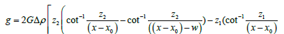
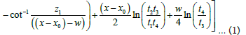
Proper forward modelling is a necessary step before carrying out inversion technique. Although 3D models are more similar to real geological model but due to complexity of the calculation, 3D models are often approximated as a number of 2D profile models. Sometimes in exploration study 2D models are taken due to simplicity and to reduce the computational time. Interpretation of gravity anomaly due to complex geological structure is not so easy, for this some basic geometrical structures are taken and gravity anomaly due to them is calculated [1,63-65]. Rectangular Prism is one of the basic geometries and it is generally used to approximate the several complex geological formations and their associated structures. A synthetic model of a 2D prism of width w in the subsurface is shown as a Figure 1. Where, x0 is the position of the prism, depth to the top of the prism is z1 and depth of the bottom of the body is z2. In such case of the synthetic model, a gravity anomaly can be computed over the surface at some observation point P given by -
t1 = (x − x0)² + z1² … (2)
t2 = (x − x0)² + z2² … (3)
t3= ((x − x0)-w)² + z1² … (4)
t4= ((x − x0)-w)² + z2² … (5)
Where, g is gravity anomaly, G is the Gravitational Constant (6.67 × 10⁻¹¹ N.m2.kg-2), Δρ is density contrast in kg/m3, and x0 is the position to the centre of the prism.

Figure 1: A rectangular prism is shown in the subsurface. Location (x0) is defined by the x position of the midpoint of the prism. Gravity value at (P) a distance x from x0 is shown here. The vertical component of gravity gz is calculated and shown.
Inversion problem formulation
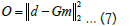
To calculate the gravity anomaly due to a sedimentary basin, density and depth profile are the most important model parameters. In this work density is obtained from other geophysical method like logging and borehole data. The main objective function, the value of which is reduced during the process is the misfit of the data value using a basic inverse problem that can be expressed as:
d = Gm+ n … (6)
Where, d is the data vector, m is the unknown model parameter vector, G is forward operator which relates model and data vector, n is additive noise. Therefore, a generalised objective function can be defined as a least square function using:
Where, m is the model estimated from inversion.
Machine learning or artificial intelligence techniques performs based on supervised and unsupervised learning. Unsupervised learning uses unlabelled input data to discover information and reveals the hidden pattern in the data. It is used mostly in categorization problem like lithological variation [66-68]. In the other hand supervised learning uses labelled data to initiate the learning from previous input output relation. Unsupervised learning requires training data to learn from relation between the input-output to produce new set of output. In machine learning approach, the forward operator G may be unknown and generally represented by a black box in the mathematical computation. In this approach the inverse problem can be slightly different from equation 7 and described as:
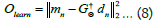
Where Θ is the parameter set, which is optimized at the time of learning process. G†Θ is the pseudo inverse operator [69]. In neural network approach, an inverse mapping is done from data to model space. It uses a non-linear basis function made up of weights and biases. Weights and biases in the layers are the pseudoinverse operator and learning occur by determining the weights and biases, which are equivalent to parameter set Θ .
Deep Neural Network (DNN) and its structure
Artificial Neural Network imitates the working function of biological neural network. Biological nervous system has cells, called neurons which are connected with the help of axon and dendrites [70]. The connecting region of axon and dendrite is called synapses that depicts a biological system as illustrated in Figure 2a. A biological neuron receives input signal from other neurons by synaptic connection of dendrites and axon terminals. Attenuation of the signal is depending on the distance from synapse to soma (main cell body). This soma processes the input signal and the output signal is transmitted through axon to the next neuron. As human brain is capable of doing complex work, intelligent machines are made in a way it simulates the working procedure of human brain. First artificial neuron was proposed by McCulloch et al. [71]. The mathematical neuron also behaves in the similar manner as the biological neuron as shown in Figure 2b with their basic architecture for a single layer Artificial Neural Network (ANN). An Artificial Neural Network is an assembly of nodes and weights, which took the input information and process it with the help of weights. The weighted sum of the inputs is fed to the transfer function (activation function) and output is obtained at output layer and applied in several geophysical application [72]. Network learning is occurred by changing the weights of the connecting neurons. Sometimes an extra free variable named bias is also added, it is like a weight which connect to a fixed input.

Figure 2: (a) A schematic diagram of biological neuron and synaptic connection. (b) Representation and workflow of a mathematical neuron. x1 to x6 are the inputs which are going to a summing node with corresponding weights w1 to w6. A fixed bias is also given. The output of the summing node is passed to the activation to get the output.
Basically, an Artificial Neural Network has 3 layers as Input layer, Hidden layer, and Output layer. Artificial Neural Network (ANN) with no hidden layer is the simplest kind and it’s called Single layer Perceptron. This is also called shallow neural network on the other hand Artificial Neural Network with hidden layer is called multilayer neural network or Deep Neural Network (DNN). It is obvious to understand that more hidden layer deeper the network as shown in Figure 3 as a multilayer feedforward network. ANN is a nonlinear system so it can solve any non-linear problem easily and is called universal approximator because it can determine the input output relationship by learning through examples, even if there is no deterministic relationship available. In neural network optimization various problems may arise and overall performance may not be as expected. It can result from incorrect network configuration, selecting poor training set (bad and overtraining), network can be trapped in local minima [73]. As shown in Figure 3, there are 6 input nodes, and each have weights corresponding to them. Each input is multiplied with its corresponding weight and they are summed up. The output of the summing node is given by:
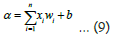
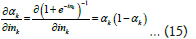
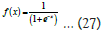
Where α is summering node, x is input, w is weights, b is bias, and n is 6 as total number of input nodes. Summed output is then fed to the activation node and the output f(α) is obtained after the activation. This can be treated as input to the next layer in the case of multilayer perceptron and so on. There ANN takes the input as nodes multiply it with the weights then sum it at each node and passes it to the next layer with proper activation and continue the similar process for the number of hidden layers until it comes to the output layer [74]. Linear activation function is the simplest kind; however, it can’t solve complex nonlinear problems, but still used to predict any quantity. For solving complex problems nonlinear activation functions are required. Sigmoid is the most popular activation function among all because it is continuously differentiable and monotonically increasing and has nonnegative and non-positive first order derivative and its output varies from 0 to 1. In order to use stochastic gradient descent with backpropagation of errors to train deep neural networks a linear like activation function is needed, but it has to act like a nonlinear function to deal complex model data relationship. In such case RELU or Rectified Linear Unit is also used as activation followed by a number of activations functions [75], to be used as per the complexity of the optimization problem as shown in Figure 4.

Figure 3: Basic architecture of multilayer feed forward neural network as first layer of input with two hidden layer is shown.

Figure 4: Various activation function and their mathematical expression.
Optimization and network training process
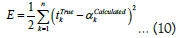
During neural network process, a network activation goes forward to produce the output and error propagates backward to optimize the result [76,77]. Once network configuration is finalized, the weight distribution must be optimized in order to minimize the cost or error function. Cost function is the misfit between the observed and true value, it describes how poorly the current model is working as an optimization process. By minimizing the loss, the network is trained to perform better. There are many optimizations techniques among which the gradient descent is one of the best optimization algorithms used to train neural network [78]. It finds the set of input variables for a target function to minimize the function value. It involves the calculation of the gradient of the target function through their slopes and measures how much the output of a function changes with the change of the input [79]. It calculates the change of the variable with the change of another model parameter as a function whose output is the partial derivative of a set of parameters of the inputs. With the increasing value of the gradient the slope steepens and correspondingly generate the optimized results. In order to compute, the slope of the function is calculated first at a point and then the algorithm is moved to the opposite direction on increasing slope. Finally, the error propagates through the hidden layers by using gradient descent approach for the training samples [80]. Most of the neural network process offers three different kind of gradient descent variants in form of Batch Gradient Descent, Mini Batch Gradient Descent, and Stochastic Gradient Descent [81]. In Batch Gradient Descent, all the training samples are passed through the network in one instance. Average of all the gradients of the samples is taken into consideration and used to calculate the new network parameters. In one epoch only one gradient descent step is present. It is good for relatively less complex error function. In Stochastic Gradient Descent only one sample is given to the network at one time. When there is a huge dataset, it is feasible to use one sample to calculate the gradient descent and increases the learning duration of the network [81]. To implement the vectorise example, ANN uses the stochastic gradient descent and Mini Batch Gradient Descent. Here a batch made up of few data samples are used to calculate the gradient.
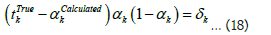
In this present study, the Stochastic Gradient Decent is considered as optimization technique which implicitly minimize the error by propagating it in the backword direction. This process is called backpropagation technique in learning network. Backpropagation is a method to calculate the gradient of the error function or cost function with the help of chain rule, whereas stochastic gradient descent is used for learning using those gradients. Gradients calculated by backpropagation describes the change in error with the change of network parameters [82]. Small change in negative gradient will decrease the error in every iteration. Let’s say the output of the network as shown in Figure 2b is αCalculated and actual output is given by mTrue. So, error in the output is e = (mTrue- αCalculated). In this regard, a cost function may be derived for gradient calculation and is generally given by sum squared error as below where the factor is taken to simplify the calculation:
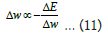
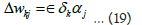
Once the parameters of the network is set the training of the network initiate the learning process. Training is a process in which the network learns the relationship between input and output by adjusting the network parameters. It happens by minimizing this error, which takes place by adjusting the weights. It will be decided in the training process that it should increase the weights value or decrease it from the previous one through iterative scheme. During the whole learning process change in weight is given by:
In more generalised form of input layer, hidden layer and output layer denoted by subscript i, j, k. So, change in weights of output layer becomes:
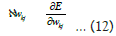
The value of the partial derivative will be calculated by chain rule:
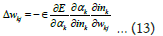
Here, Δwkj is the weight change of output layer, ϵ is the learning rate, ∂E is the change in error, ∂αk change in the activation of output layer, ∂ink is the change in the input of the output layer.
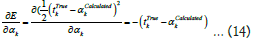
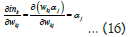
Putting these values in equation (13), the value of change in weights as

Therefore, the change in weight in input to hidden layer is also calculated by the help of chain law as;
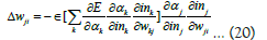
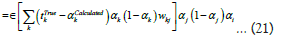
Replacing this value in equation (20),
So, updated weights are
wkj = wkj + Δwkj … (25)
wji = wji + Δwji … (26)
This optimization process is called supervised learning. If the error remains high and flat for a time being then it suggests that the training is stuck into a local-minima. It now requires a new set of initial guesses to restarts the training. If the network is well trained, then it offers a result very fast. The whole learning process of deep neural network in illustrated through a flow chart in Figure 5.

Figure 5: Flowchart showing the neural network algorithm used here.
Conventionally, the gravity anomaly for any sedimentary basin can be assessed from a depth section and distribution of lateral/ vertical density information. Finally, it is carried out by specifying a set of approximate depth to the density interface by using the prior information. In this theme of results and discussion, firstly a prismatic model is considered to evaluate the gravity anomalies and their associated model parameters followed by synthetic subsurface model of depth profile using prismatic approximation and later the computational inversion algorithm is applied to a real data.
Single 2D prism
In the present study of an inversion problem, the input in the neural network is considered as a gravity anomaly for a prism for simplicity and later it was used to approximate the complex sedimentary basin. So, the number of nodes in the neural network is equal to the total number of observation points and the output is the model parameters of 2D prism (position x0, density contrast Δρ, depth to the top of the prism z1, depth to the bottom of the prism z2). The weights and biases are taken randomly between 0 and 1. Then the inputs are multiplied with the weights and summed according to the above said equation 9 to propagate the summation through a nonlinear transfer function called sigmoid function given by:
Through the process of error propagation, the network learns the characteristics of the problem and trained its network of perceptron to deliver the results. The artificially created neural network is trained with a large number of data sets which were created by considering different sets of model parameters based on the priory information. Then the network learns the relationship between the input and output and train it to give the desired outcome. Artificial Neural Network is evaluated by using root mean square error between the network output and the desired output. Then the error is back propagated by gradient descent method to optimize the weight and biases followed by the testing of the network by using the actual dataset. Finally, it converges to the optimized results as a model parameter which highly depends on the space dimension of unknown parameters [83].
Gravity anomaly due to a single prism is obtained from the formula given in equation 1 and the pictorial representation of 2D prism with anomaly is illustrated in Figure 6. It is evident from Figure 6 that maximum anomaly is observed exactly at the top of the prism when the dip of the prism is basically zero. To optimize the model parameters of 2D prism, a deep neural network with 120 input nodes, 30 hidden layer nodes and 5 output layer nodes corresponding to 5 model parameters are generated. A total of 6 different sets of training data is used to train the network. These sets were created from 6 different sets of model parameters in the vicinity of priory information. For real dataset, a vast range of model parameters should be taken to create the training dataset to train the network. To initiate the training, the gravity values obtained from synthetic computation of 2D prism are normalized between 0-1. To train the first layer of network, sigmoid function is used as activation function and linear activation function is used for the output generation at the output layer through learning occurs by backpropagation of error. Stochastic gradient descent is used as the optimization process to reduce the error.

Figure 6: (a) Gravity anomaly in mGal due to a single rectangular prism (without noise) and (b) with noise. (c) The prism is plotted below the
subsurface just with anomaly for better understanding, (d) Gravity anomaly curve showing the actual and inverted anomaly for noiseless single prism
data. Blue star is showing the real data and red circle is the inverted anomaly data and (e) Anomaly curve with contaminated noise of 5% Gaussian
Noise. (f) Root means square error vs iteration curve showing the minimization of the error while training the network for single prism. 

After completion of training, the network testing is done with the synthetic dataset and inverted anomaly is obtained. Now the network is trained to give desired output. To assess the model’s robustness against the noises, 5% of Gaussian noise is added to the anomaly as shown in Figures 6a and 6b. Figure 6d shows the actual and inverted anomaly for datasets without noise and Figure 6e with noise contaminated datasets of single 2D prism. Here misfit in the model parameters is taken as cost function and it is minimized during the training of the neural network. The error got minimized during the training at very low learning rate. At first the error was high and after training and changing the network weights accordingly the error is reduced close to zero at around 200 iteration as shown in Figure 6f. By training, the neural network learns the relationship between the input and output using gravity anomaly and model parameters and finally converges to the real model parameters in terms of density, position, width, depth of the top and bottom of the prism as output. The gravity anomaly was given as input at each node and each output node give each parameter as output. After inversion the error in the gravity anomaly for noiseless data is 2.923775 × 10⁻⁸ and for noisy data it is 5.341200 × 10⁻² and the comparison of the generated model parameters versus real parameters for a single 2D prism are shown in the Table 1.
| Model parameter comparison for real and calculated values | ||
|---|---|---|
| Noise free data | ||
| Real values | Calculated values from inversion | |
| Position of the prism (x0) | 0 | 1.696030 × 10⁻⁷ |
| Density of the prism (p in kg/m3) | 200 | 200 |
| Width of the prism (w in m) | 800 | 800 |
| Depth of the top of the prism (z1 in m) | 900 | 900 |
| Depth of the bottom of the prism (z2 in m) | 2100 | 2100 |
| Data with 5% Gaussian noise | ||
| Real values | Calculated values from inversion | |
| Position of the prism (x0) | 0 | 1.696040 × 10⁻⁷ |
| Density of the prism (p in kg/m3) | 200 | 200 |
| Width of the prism (w in m) | 800 | 800 |
| Depth of the top of the prism (z1 in m) | 900 | 900 |
| Depth of the bottom of the prism (z2 in m) | 2100 | 2100 |
Table 1: The model parameter comparison for both noisy and noiseless data calculated for single rectangular prism.
Synthetic layer generation and depth profile
The developed DNN approach of gravity inversion algorithm described in the earlier section is utilized here by using synthetic data from a complex sedimentary basins. Here two different types of synthetic examples are considered as Model 1 and Model 2. Model 1 has a complex sedimentary basin with constant density and variable depth as shown in Figure 7 where Figure 7a demonstrate the model 1 without noise and Figure 7b with contaminated noise of 5% of Gaussian noise. Whereas Model 2 has again much more complex sedimentary basin relief with depth varying density contrast as shown in Figure 8 where Figure 8a demonstrate the model 2 without noise and Figure 8b with contaminated noise of 5% of Gaussian noise. The total length of the profile is 6000 m along the x axis transverse to the strike of the sedimentary basin with 300 equispaced observation points with 20 variable rectangular prisms. The profile is assumed to have a constant density contrast of lateral and vertical density variation at the basement depth interface across the profile containing 20 prisms. Then the model is simulated for the training for a maximum number of generations of 800 based on the desired accuracy of close to real values using the depth bound of the model [24]. Afterward, model is trained with a vast number of synthetic data, through which we observe that the objective function values converge within a maximum of 600 runs and error plot is shown in Figure 9. In a similar fashion, model parameters are inverted using gravity anomaly for a complex synthetic sedimentary basin where lateral and vertical density variations are assumed to relate with real geological scenarios and the model is shown in Figures 8a and 8b without and contaminated noise correspondingly. Error for both noisy and noise free data is shown in Table 2. From the table it is vital to note that that the error increases with increasing parameters though the range of error is not so significant for the consideration (Table 3).

Figure 7: (a) Anomaly curve comparing actual and inverted anomaly for synthetic layer (Model 1 with constant density). The synthetic layer is plotted
just below the surface. (b) Anomaly curve comparing actual and inverted anomaly for synthetic layer with 5% Gaussian Noise where blue colour curve
denotes the actual value and red colour shows the inverted result. Complex sedimentary layer is shown in the lower part as a combination of 2D
prism. 

Figure 8: (a) Anomaly curve comparing actual and inverted anomaly for synthetic layer (Model 2 with heterogeneous density). The synthetic layer
is plotted just below the surface. (b) Anomaly curve comparing actual and inverted anomaly for synthetic layer with 5% Gaussian Noise where blue
color curve denotes the actual value and red color shows the inverted result. Complex sedimentary layer is shown in the lower part as a combination
of 2D prism. Density contrast for the calculation is taken as Δρ (z)=(-0.8+0.7174z-0.229z2 ) × 1000 kg/m3. 

Figure 9: Root means square error vs iteration curve showing the minimization of the error while training the network for model 2 od complex sedimentary basin with density variation along depth section.
| Error in gravity anomaly for noise free and noise data after inversion (Model 1) | |
|---|---|
| Noise free data | 6.2534 × 10⁻⁸ |
| Data with 5% Gaussian noise | 0.2599 |
Table 2: The comparison of error in gravity anomaly for noisy and noiseless data for synthetic layer (Model 1).
| Error in gravity anomaly for noise free and noise data after inversion (Model 2) | |
|---|---|
| Noise free data | 7.8034 × 10⁻⁸ |
| Data with 5% Gaussian noise | 0.3675 |
Table 3: The comparison of error in gravity anomaly for noisy and noiseless data for synthetic layer (Model 2).
Real example: Sayula Basin, Mexico
The DNN is trained with both noisy and noiseless data in three different cases of the synthetic models to deliver significant and satisfactory results with visibly small error. Further, to examine the developed approach with true case, the example with real field data is taken from residual Bouguer gravity anomaly profile across the Sayula basin from south central Mexico. The basin fill mainly consists of basic lava, tuff, and breccias as shown in Figure 10a. The entire 16 km gravity profile has been digitized from García- Abdeslem et al. [84], with 101 equally spaced data points. Total length of profile is divided into 101 gravity data points and a total of 750 infinitesimal small rectangular prisms with constant width were taken to recreate the basin structure synthetically with lower and upper bound range of 0 m to 5000 m. The density contrast decreases with depth and follows a depth varying density contrast relation with each and every individual prism. To simplify the calculation, we considered the depth value of the midpoint of the prism to calculate the density contrast. Then the gravity value of the basin is created using the previous mentioned relationships, and used as the training dataset. The formula to calculate the density contrast is taken as:


Figure 10: (a) Geology map of Sayula Basin, Mexico, (b) Anomaly curve comparing actual and inverted anomaly for Sayula Basin, (c) Error curve for
the final convergence to output parameter. 


Then the network is trained with a training dataset, which were created by using convenient parameters. The network is trained to give the basement depth value using 750 number of nodes in output layer to calculate the depth as the output of the network through a supervised learning process. The network is trained from the sample data values given for a different basement depths of having different density variations with depths. Further, the trained network is subjected to the real data and the depth values are obtained. The real and inverted gravity anomaly is shown in Figure 10b with real and inverted depth profile in blue and red color. Except for a small region the inverted data is matching the real anomaly. The optimization error curve of gravity anomaly for the Sayula Basin is shown in Figure 10c. After the optimization with the maximum iteration of 180, the RMSE in gravity anomaly for the best inverted model is close to zero. The maximum depth of the sedimentary basin is around 1000 m, and it is very much similar to the result obtained by García-Abdeslem et al. [84]. It is important to note from the error curve shown in Figure 10c that initially the error is about 1400 but soon after 100 itertaion when the network is trained, suddenly the behavior of error curves saturate to 0.6270 i.e., close to zero [85].
Deep Neural Network approach is applied to investigate the depth profile of a sedimentary basin having a complex density behavior. Determining the appropriate basement relief of any complex sedimentary basin from the gravity anomalies can be solved using this approach much faster with unbelievable accuracy without any constrain. The developed algorithm of DNN is based on the stochastic gradient descent optimization approach using backpropagation error scheme. It requires significantly enormous datasets to train the neural network to achieve the desired accuracy. The entire basement relief of any complex sedimentary basin along any profile can be subdivided into an infinitesimal tiny segment of rectangular prism to approximate the basement topography and assigned the lateral as well as vertical density variation to each segment of prism. It is also emphasized that the present approach of DNN work perfectly well with any sedimentary basin having constant as well as lateral and vertical density variations. We presented the three cases of synthetic model from simplest model of prism to complex model of synthetic sedimentary basin to show the efficiency, reliability and stability of the presented approach. The inversion algorithm recovers the depth to the basement of the formation and overcomes the drawback of nonlinearity and local convergence without any complex mathematical relationships. It also provides the best continuity of the basement interface using prismatic approximations as compared to traditional approaches due to its design to mimic the human brain, so it continuously improves itself in order to deliver better results. Finally, the whole procedure of training network using DNN is verified with real data from Sayula Basin, Mexico. The inverted depth interface and basement topography offer reasonable results and show a good agreement with reported results from earlier studies.
We thank the Director, NCESS, and the Secretary, MoES, Government of India, for providing the funds and unconditional support to carry out this work. One of the co-author MM is also thankful to Director of IIT (ISM) Dhanbad, and Head of the Department of Applied Geophysics and all teachers for their support and teaching during this dissertation time. We are grateful to the editor and anonymous reviewers for their thoughtful suggestions over the manuscript.
All generated data and developed MATLAB based computational codes can be provided after a special request to the corresponding author.
Citation: Dubey CP, Majhi M, Pandey L (2023) Basement Relief of Sedimentary Basin Using Gravity Data from Deep Neural Network Approach. J Geol Geophys. 12:1109.
Received: 26-Apr-2023, Manuscript No. JGG-23-21564; Editor assigned: 28-Apr-2023, Pre QC No. JGG-23-21564 (PQ); Reviewed: 12-May-2023, QC No. JGG-23-21564; Revised: 19-May-2023, Manuscript No. JGG-23-21564 (R); Published: 26-May-2023 , DOI: 10.35248/2381-8719.23.12.1109
Copyright: © 2023 Dubey CP, et al. This is an open-access article distributed under the terms of the Creative Commons Attribution License, which permits unrestricted use, distribution, and reproduction in any medium, provided the original author and source are credited.