Fisheries and Aquaculture Journal
Open Access

Assessing the Exploitation Strategies of the Shrimp Fishery in the Gulf of California

Hugo Gael Ram�?�?�?­rez-Villalobos and Ernesto A. Ch�?¡vez^{* *}Correspondence: Ernesto A. Chávez, Interdisciplinary Center of Marine Sciences (CICIMAR), IPN. Av. IPN s/n Col. Playa Palo de Sta. Rita, El Conchalito, La Paz, BCS 23096, Mexico, Tel: +52 612 120 3845, Email: ,

Author info »

Introduction

The world shrimp production for fishing and aquaculture is around 6.4 million t of whole shrimp and represents an annual income of more than 20 billion dollars [1]. In Mexico, shrimp is the most valuable fisheries resource, representing almost 40% of the total value of the fisheries production landed and a total value of more than US $ 132 million per year. Shrimp fishery provides with more than 30,000 direct and indirect jobs [2,3]. The shrimp fishery in the Mexican Pacific is supported mainly by four peneid shrimp species, commonly called as follows: brown shrimp Penaeus californiensis, blue Penaeus stylirostris, white Penaeus vannamei, and red or crystal shrimp Penaeus brevirostris. The total wild shrimp production was 74,000 t for the Gulf of California in 2013 [3,4]. The proportion of species caught in the eastern Gulf of California is varied depending on the habitat, region, and depth. For the southern Gulf of California (southern Sinaloa), the inshore water is dominated by white shrimp (89%) and followed by blue shrimp (11%). At the offshore area, the main species is brown shrimp (55%), followed by white (41%) and blue (4%) [3,5]. Globally, brown shrimp dominates catches with 70-80% of total production [6]. The offshore fleet based in Mazatlan captures 70% of their shrimp catch in the central and north of Sinaloa throughout the fishing season.

The shrimp fishery is also the most controversial and problematic in the country. There is a strong debate about the level of exploitation and the present and potential effects on the ecosystem, mainly due to the high levels of effort and overcapitalization of the industry, detected since the early 1970s [7]. Trawling equipment has been intensively in use for the past 60 years, which is recognized as one of the most ecologically aggressive [8-10]. According to official statements [5,11], the shrimp fishery of this region shows symptoms of overcapitalization and strong competition between the private and social sectors for the resource. All of these statements justified doing an assessment of the fishery, in order to determine whether the fishery is under or overexploited as a primary goal of this research and to define management actions that should be adopted to make it more efficient, addressing the fishing effort and the ages of first catch toward the optimum yield.

Materials and Methods

Study area

The Gulf of California (GC, Figure 1) is a marginal sea that communicates with the Pacific Ocean through a mouth 220 km wide. It is located between 208 and 328 north and 105.58 and 114.58 west in the Eastern Pacific, with an approximate length of 1,100 km [12]. In the southeastern part of the GC, the most important fishing harbors are Guaymas in the State of Sonora, and Topolobampo and Mazatlán in the State of Sinaloa.

Figure 1: The Gulf of California, study area.

Catch data

Catch data of official records are available on the official website [13,14], in the section on statistical information, by species and entity. It contains information from the years 2006 to 2014 and the statistical yearbook of fishing and aquaculture of the years 1997-2013.

The fishing boats

The industrial offshore fleet exploits preadults and adult shrimp in open waters, with vessels longer than 10 m in up to 40-day trips, using trawl nets. The crew is composed by seven members per boat. The two most important landing harbors are Mazatlan and Guaymas, on the eastern coast of the Gulf. Engines usually have 425 HP, consuming 53 l/hour or approximately 1,280 l per day. During the last 14 years, the number of boats ranged from 1,422 in 2003 and 2004, decreasing to 755 in 2013. This trend is a result of management regulations addressed to make the fishery more profitable.

In September, only three vessels based in Mazatlán were reported in the fishing grounds. In October, the number of vessels increased considerably to 567 boats, and in this month the trawling boat reached its highest number. In November, the number of boats in the fishing grounds decreased slightly to 555, and declined to 292 in March (Figure 2).

Figure 2: Number of fishing boats of the south GC, working every month. Fishing season 2011-2012.

The fishing grounds

The shrimp fleet located in the states of Sinaloa and Sonora is the largest in the country, with more than 700 vessels. This fleet has influence throughout the continental shelf from the Gulf of Tehuantepec in southern Mexico, to the upper GC and off the coasts of Ensenada, on the northwest side of the Mexican Pacific. Thanks to the satellite monitoring data of these vessels, it was possible to determine accurately the fishing areas swiped by each boat. These data were sorted to obtain only those from the southern Gulf of California. The following debugging step was made by selecting trawling speed; according to the literature, the vessels trawl at speeds between 2 and 3.5 knots. Later, maps were created with the aid of the surfer software, as shown in Figure 3, evidencing the dynamics of the fishing fleet. At the beginning of the season, the majority of the boats keep trawling close to the coastline; in September, they are found only along the coasts of Sinaloa and Sonora. For October and November, they increase their mobility moving to the south of the GC, to the upper gulf, and a bit to the Pacific coast of the Baja California peninsula. In December, the boats begin to move away from the coast, where many of these boats are adapted to perform another type of fishing activity, catching other species of commercial interest, such as shark and scale fish. In March, the number of shrimp boats decreases considerably since the shrimp biomasses decrease and the closed season approaches.

Figure 3: Dynamics of the shrimp fishing fleets over the season. Based on GPS records of the fishing boats.

Stock dynamics and assessment

The population growth parameter values are from previously published sources (Table 1).

Table 1: Age and growth population parameter values of three shrimp species of the GC. (W in g; L in mm)

Unfortunately, no recent population parameter values are available in the literature, so it is assumed that the values in Table 1 are valid. However, it has been suggested that “empirical weight-at-age approach is best applied to data-rich stocks for which growth is a difficult process to characterize” [15-17]. Estimates of growth rate, length–weight relationship, and natural mortality are necessary to transform catch data into number of organisms by age. With the values of the von Bertalanffy growth parameters and the allometric equation that defines the length–weight relationship, the model was used for assessing and simulating the fishery. This is part of the previous knowledge required for the stock assessment and management [18,19], and the magnitude of cohorts depends on the von Bertalanffy´s growth parameters, the age structure and the recruitment rates [20].

Parameters of each shrimp population, together with the catch data, were analyzed with the simulation model FISMO [21,22]. The simulation model reconstructs the structure of ages over time, which allows simulating exploitation scenarios under different combinations of fishing intensities and age of first capture to maximize biomass, capture, and profits. The analytical procedures adopt the concepts and points of view of [21-24]. The model was written in excel. A matrix of population numbers per age group, and weight of each age class was assigned for each year of the catch data series. After the age of first catch (tc) was defined, the catch equation was applied to each age class. The difference between expected and recorded catch was minimized with the aid of the “goal seek” function to determine the fishing mortality value (F). The macro developed for this purpose determined the F value year by year. In this manner, the model was fitted with a series of catch values, represented by the numbers and weights per age. The shrimp numbers for each age class every year were determined with the aid of the recruitment model [23,24]. Once the model was fitted, it was possible to simulate exploitation scenarios by just changing the F and the tc that would represent the simulated status of the fishery.

Catch data were transformed into numbers by age group, allowing estimation of the age composition of the catch. The total mortality (Zt) was determined with the exponential decay model as follows:

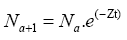
where N_a+1 is the number of organisms of the age of a+1 and Na is the number of organisms of age a in the age groups and reconstructed using the potential regression for the estimation of parameters a and b such as follows:

P = aL^b

For the estimation of natural mortality (M), the criterion proposed by [25,26] was adopted, where M 5 1.5 K. In the exploited age groups, the fishing mortality (F) is added to the M, so that Z 5 M 1 F. For the adjustment of the variables of the initial state, the abundance by age class (Na, y) was defined by using the abundance by age Na/ΣNa obtained from the equation.

In the following years, the age structure was defined after estimating the number of one-month-old shrimp, called recruits here, with the recruitment model [23]. These values were used to calculate the catch per age as proposed by [27] and that have been integrated into the simulation model FISMO [21,22].

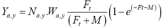
where Y_a,y is the capture of shrimps of each age; N_a is the number of shrimps at age a in the year y; W_a,y is the weight of the shrimp equivalent to N_a; F and M were described in the previous paragraph. Given the initial conditions established, the values of Y_a,y, can be adjusted by varying the initial number of recruits and linked to the equations described earlier until the condition of the following equation is met:

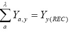
where Yy _(REC) is the catch recorded during the year y, a 5 age of first capture (years), and tλ 5 3/K or longevity, where K is the growth constant of the von Bertalanffy equation, for example, tλ 5 2 years, a value found assuming a reasonable life expectancy. L_max is when 95% of the population reaches 95% of L∞, the asymptotic length. Therefore, making L_max 5 0.95L∞ in the von Bertalanffy rowth equation and finding the respective value of t, the value of the longevity is found. The catch equation was applied for each year in the time series analyzed. The estimates of the population biomass and the exploitation rate E 5 [F/(M 1 F)] was made for each age class in each fishing season with the help of the model. These values were compared with the E value at the maximum sustainable yield level (F_MSY). Next, a diagnosis was made for the years in which the populations have been overexploited, providing a way to make recommendations for a new increase or decrease of F in the fishery.

To provide some robustness to results, estimations of the coefficient of variation between recruits one year and the number of adults the year before were made, as well as the coefficient of variation (CV) of the simulated catch (Table 2).

Table 2: Mean values and Coefficients of variation (CV) of simulated catch (t), the number of adults next year, and the number of recruits one year before, during the 30-year simulation period. Values were estimated for the three species of shrimp caught in the GC.

Results

The most abundant species are the brown and the blue shrimp. The catches of these two species were similar ranged 4,000-8,000 t per year in the years from 1997 to 2005. White shrimp landings did not exceed 2,000 t per year. In 2006, the brown and blue shrimps decreased, and the white shrimp had a slight increase. In the next three years, the catches of the brown and blue shrimps remained stable, and increase again since 2010 when white shrimp landings were relatively low. However, in general, the shrimp total catch increased until reaching its maximum around 36,000 t in 2013. This value represents five times of the landings of the year 1997 (7000 t only, Figure 4). This increasing trend is somehow confirmed by shrimp samplings during the closed season [23].

Figure 4: Shrimp catch by species and in total (1997-2014) at the southern GC.

Shrimps have high growth rates. The brown shrimp had a growth constant K of 2.23 with a maximum length of 24 cm and a maximum weight of 264 g. Their maximum age is about 1.2 years (Figure 5). The age of sexual maturity reported for this species is four months at about 13 cm of total length and a weight of 40 g, which is coincident with its size at first capture (tc).

Figure 5: Growth rate of the brown shrimp, as described by the von Bertalanffy growth model. A length (cm), B weight (g).

Blue shrimp is the second most important stock in the shrimp fishery of the southern GC. They had a growth rate K similar to that of the brown shrimp, and reaching their maturity at the age of four months, with a weight of 40 g and length of 12 cm.

Brown shrimp

The analysis of 15-year (2000-2014) data shows a constant catch in all the period, and the catch reached its maximum 16,013 t of live weight in the year 2013 in the southern GC (Figure 6). The average catch was around 7,500 t per year. The biomass remained quite constant until 2009, when high catches were recorded, followed by a decline since 2009. However, the highest catch recorded in 2013, and the decrease of the stock biomass is interpreted as effect of the fishing intensity on the stock size. The fishing mortality at the maximum yield level was estimated to be FMSY 5 0.2, which was higher than all the F values in the previous t years (Figure 7), suggesting that the fishery was underexploited during all previous years.

Figure 6: Stock biomass and catch of the brown shrimp (Penaeus californiensis (Holmes, 1900)) 2000-2014 in the southern GC.

Figure 7: Trends of the fishing mortality F and the exploitation rate E of the brown shrimp fishery in the southern GC for the years 2000-2014.

Blue shrimp

The catch increased from 3,183 in the year 2000 to 7,150 t in 2005, and decreased in 2006 and 20006 to its lowest only 3,000 t. However, the catch increased again after 2007 and reached its highest 14,418 t in 2011. The catch fluctuate 2150-3508-19-273 ed around 10,000 t since 2012.

The estimated stock biomass was relatively high above 400,000 t before 2010, and decreased to 250,000 t during the last four years, indicating that the decline in biomass might have been caused by the increasing fishing intensity in these years (Figures 8 and 9). This indicated that the stock was probably overexploited during the last four years of the data series.

Figure 8: Catch and stock biomass of the blue shrimp (Penaeus stylirostris Stimpson, 1874) stock of the southern GC during the years 2000-2014.

Figure 9: Trends of the fishing mortality F and the exploitation rate E of the blue shrimp stock in the southern GC for the years 2000-2014.

The comparisons between the estimated F and E with those values at the MSY level indicated that at least the blue shrimp stock was overexploited in the years 2011 and 2013.

White shrimp

From year 2000 throughout 2008, catch of this species showed an increase trend with a maximum catch about 2,000 t. It dropped to only 180 and 194 t in 2009 and 2010, respectively. In 2011, the catch increased again approaching 2,000 t, but decreased to 485 t in 2012. However, in 2013, the catch of this species jumped to 6,402 t, and remained at a similar high level in 2014 (Figure 10). From 2000 to 2012, fishing mortality on this species was very low. However, the increased fishing mortality in both 2013 and 2014 might have resulted in the overexploitation of this species (Figure 11). It is similar to those of the two other species, which also showed that the fishing mortality might have resulted in the overexploitation of the shrimp stocks in recent years.

Figure 10: Catch and stock biomass of the white shrimp (Penaeus vannamei Boone, 1931) stock of the southern GC during the years 2000-2014.

Figure 11: Trend of F and E of the white shrimp stock in the southern GC for the years 2000-2014.

Discussion

Exploitation of shrimp in Mexican waters is under the Official Mexican Regulation NOM-002-SAG/PESC-2013. Among the current regulations, there are closed seasons, restriction to exploitation in some areas, restriction of the fishing effort, and regulation on the use of fishing gears. In Mexican waters, the shrimp fishery is the most important for its value. Shrimp catch in the Pacific coast represents 86% of all Mexican shrimp, and the landings of the GC amount to 80% of all shrimp caught in Mexico.

Catch data display an annual increase for the three species in recent years, having the brown shrimp as the most abundant in 2014, with 48%, followed by blue shrimp with 34% and white with 18%, in the offshore catch by the fishing fleet in the southern part of the GC. These proportions have been rather constant over time.

High catches landed in the last few years might be caused by high exploitation rate, which might have reduced the tock biomass and have caused the overexploitation of the stocks. According to the Fisheries Institute of Mexico (INP), the main factors responsible for this situation are high fishing capacity, lack of control of fishing effort, and a strong impact of trawl nets on the fishing grounds [6-10].The shrimp fisheries in the tropics are considered as non-sustainable from the economic, social, and environmental viewpoints [28-30]. However, our results here do not confirm this; by the contrary, shrimp stocks of the GC have shown high resilience toward the fishing pressure, and their high turnover rate, determined by their fast individual growth, high recruitment rates, and very high fecundity compensate high mortality values caused by natural factors and fishing pressure [30]. They should sustain that way as far as the fishing pressure does not grow to excessive limits. Usually, when the condition of a non-profitable activity can be attained before the stock biomass is exhausted.

Similar to other fisheries, historic trend of shrimp fishery in Mexico has passed through several steps. It started with high yields and low fishing pressure. After some time, with an increasing demand, the fleet size increased with better technology, until the maximum yield is attained and even surpassed, which resulted in the overexploitation of the stocks [31]. In a study of the fishery at the south GC [30], it was indicated that management plans, knowledge, and attitude of the fishers should be integrated to improve the success in the management of these fisheries.

Management scenarios proposed here are based on the indicators such as the age of first capture, the fishing mortality, and the stock biomass. Evaluation of the results is based upon quantitative performance of yield and stock size, often referred to their values at MSY.

Age structure models such as the one used here, allow us to evaluate the consequences of changing the age of first capture and the fishing effort on yield and variability of the stock–recruitment ratio. They also can be used for a quantitative evaluation of the effect of F for recovering depleted fisheries [30,32,33]. In other framework, this knowledge has been used to examine changes of biomass, recruitment, and harvest rate, based on the catch data transformed into size composition data, in a similar way as [34-36].

Two fishing scenarios were identified apart from the current one (the 2014 fishing season). The first one is the MSY, while the second one is the MSY/fisherman. Several variables obtained as output after setting the reference conditions of the 2014-fishing season. This allowed a quantitative comparison on the advantages and disadvantages of each option (Table 3). The current yield sets the initial condition of the fishery, where tc, the number of boats, and the number of fishers have constant values. All other variables are different and display changes after testing different F and tc values. The best F and tc combination could be identified for the fishery.

Table 3: Management scenarios identified for the three species of shrimp exploited in the central and southern Gulf of California under different combinations of the age of first catch (tc) and the F. Scenarios FMSY and FMSY/Fisher were compared respecting to the fishing season (2014) used as reference. Stock biomass and catch values are in thousand t.

In the case of brown shrimp, its tc is four months, with F=0.22, and 15,967 t of catch. The MSY scenario increases shrimp stock size and also increases the yield to 20,889 t, with a lower F= 0.2 and a higher tc=5 months. This is a better option for brown shrimp. The MSY/ fisher scenario suggested that the stock biomass could increase to more than twice of the current value, which allowed us to obtain a high catch (16,081 t) with a reduced F (0.1) and an increased tc (five months). However, this scenario required the number of boats and fishermen be significantly reduced. Therefore, the MSY scenario with tc=5 month is the best option for brown shrimp fishery.

For blue shrimp, the current tc is four months, with F=0.14 and 11,237 t of catch. The MSY scenario showed a best option with an increased catch of 15,472 t at F=0.2 and tc=5 months. This indicated that both the number of boats and the number of fishers could be significantly increased. By contrast, when the scenario MSY/fisher is considered, and to maximize the yield per fisher, it would be necessary to reduce the fishing mortality (F=0.11) and increase tc (five months) to maintain a slightly higher catch (Y= 11,911 t).

The current catch for white shrimp is 6,098 t with tc=4 months. In the MSY scenario, the best option will be F=0.15 and tc=5 to obtain a catch of 7,343 t. This will allow to increase fishers to 7,669 direct jobs. The scenario MSY/fisher requires a reduction of F to 0.12 (601 boats and 4,213 fishers). In this case, the fishers would get 2 t per head, and the stock biomass would reach the highest value caused by a low F, implying some population recovery.

Management considerations

There are some pros and cons derived from the options just examined; therefore, managers should consider all of the management points of view, which briefly are as follows: maximizing the catch, conservation of the resource, maximizing the economic return, and maximizing the social benefit or, in other words, the number of jobs. Maximizing the catch does not necessarily mean the maximum economic benefit, because the maximum economic yield usually is met with lower F values than those required for the MSY, and after this reference point with further increase of F, the profits decline; however, this topic is beyond the scope of this paper. If the goal is the highest yield, then the MSY is the best option in the three cases. It would bring an increase of more than 10,000t in overall catch, with a small reduction of the stock biomass of the blue shrimp, and allow a higher number of direct jobs. From the viewpoint of biological conservation, the best option is to obtain the maximum yield per fisher, which requires a reduction of fishing pressure and result an increase in the stock biomass. However, this option would require a reduction in the number of direct jobs, which may be a major constrain from the social viewpoint. It might be not good to use the season 2014 as a reference because the fishery seems to be close to the economic equilibrium level. The crises of over fishing capacity in this fishery have occurred several times, forcing the fishing authority to apply more strict regulations to reduce access of the fishing grounds.

As this is a multispecies fishery, the same vessels perform the extraction of the three species with the same fishing gears in the same space and fishing grounds; therefore, it is necessary to propose an optimum management scenario for the capture of shrimp stocks. When the output lines of potential yield of the three stocks as function of F are overlapped as in Figure 12, it is evident that the total yield with tc 5 4 months is not the maximum that could be obtained. If tc is increased to five months old and the resulting trend lines are overlapped, it is evident that the line obtained after the addition of the three stocks catch, suggesting that the fishery can withstand a higher fishing pressure to obtain the maximum yield, passing from 38,000 t to 55,000 t (Figure 12). This provides a maximum yield reference value from where to explore the possibility to identify another fisheries target, like a precautionary approach, that is, 0.9MSY, which still would attain higher yields than in the current scenario (Figure 12).

Figure 12: Potential yield for each one of the three species of the shrimp fishery of the GC as a function of F. Lines of yield were overlapped and another line displaying total yield, is shown at two tc values, A) at tc = 4 months, and B) at tc = 5 months old.

Based on simulations, we recommend that regardless the scenario, increasing the age of the first capture from four to five months old (Figure 13) is a better option than the current condition; this would mean an approximate total length of 13 cm for brown shrimp, 15 cm for the blue shrimp, and 12 cm for the white shrimp.

Figure 13: Potential yield for each one of the three species of the shrimp fishery of the GC as a function of the fishing effort in days. Addition of yield values are displayed as total catch. Yield values are shown at two different tc values, A) at tc = 4 months, B) at tc=5 months old. According to this graph, with tc = 4 months, the best fishing option is attained with 10,000 days, represented in both figures as a light blue vertical line; here, maximum yield would be 25,000 t. However, with tc=5 months, a much higher effort of up to 35,000 fishing days could be applied, and the yield could be higher than 50,000 t.

In regard to the fishing mortality, the Mexican fisheries authority [37] considers that this variable keeps the fishery at the limit of sustainability and therefore recommends not to further increase in fishing effort, to reduce the fishing mortality and to standardize the fishing power of the vessels to make the fishery more profitable [38-40].

Conclusion

The simultaneous exploitation of the three species implies several constrains for the application of a uniform but necessary number of fishing permits. In the current option, the F values display a wider range; however, in the two other scenarios, F values have a narrower range between the stocks. Therefore, a convenient simplification could be the authorization of the same number of fishing permits regardless of the species target; with this option, the effect on each stock would be not quite different. If the FMSY is chosen, for practical reasons, it would be convenient to fix in 1000 the number of boats; this would imply a close performance of the fishery around the target value. However, if the option FMSY/fisher is adopted as target, a number of permits near to 530 would be recommended; this is nearly 200 boats less than the current option, which might imply a social cost hard to accept, although it would be beneficial for the conservation, because the stock biomass would increase. To avoid a negative social impact, in the meantime, we recommend to maintain a constant fishing effort and to increase the age of first catch from four to five months; the adoption of this recommendation would imply the benefit of increasing the stock biomass. Kell et al. states that “A major uncertainty in stock assessment is the difference between models and reality”; then, the criterion adopted in this analysis, a pragmatic alternative to hindsight to forecast future catch can be considered.

Acknowledgments

The Camara de la Industria Pesquera (Fisheries Chamber) in Mazatlan provided updated data of the shrimp fishery. An anonymous reviewer made valuable comments. E. A. Chavez holds a research grant from COFAA and EDI, both from IPN. This research received no specific grant from any funding agency, commercial, or not-for-profitsectors.

References

1. FAO. Anuarios de Estadísticas de pesca. Cuadros resumidos 2012. Producción pesquera: estimación del valor por grupos de especies, Rome. 2014
2. CONAPESCA. Anuario Estadístico de Pesca. Secretaria de Agricultura, Ganadería, Desarrollo Rural, Pesca y Alimentación, México City. 2012.
3. CONAPESCA. Comisión Nacional de Acuacultura y Pesca. Mazatlán, 2008b. 2013.
4. CONAPESCA. Plan de Manejo para la Pesquería de Camarón en el Litoral del Océano Pacífico Mexicano. SAGARPA-CONAPESCA-INP. 2004.
5. López-Martínez J, Hernández-Vázquez S, Rábago-Quiroz C, Herrera- Valdivia E, Morales-Azpeitia R. Efectos ecológicos de la pesca de arrastre de camarón en el Golfo de California. Estado del arte del desarrollo tecnológico de las artes de pesca. In: J. Santinelli, (ed.) La situación del sector pesquero en México. CEDRSSA. Palacio Legislativo de San Lázaro, México City. 2008;13-47.
6. Lluch-Belda D. La pesquería del camarón del Pacífico (Diagnosis monográfica de los conocimientos existentes). IPN-CICIMAR, DGINPEPES, CICTUS-UAS, Cocoyoc, Morelos. 1982.
7. Jones JB. Environmental impact of trawling on the seabed: a review. New Zeal J Mar Fresh. 1992;26:59-67.
8. Morales-Bojórquez E, Madrid-Vera J, Díaz-Uribe JG, Aguirre-Villaseñor H, Liedo-Galindo A. Distribución y abundancia de camarón café (FanfantePenaeus californiensis) en el norte de Sinaloa, México. In: López-Martínez J, Morales-Bojórquez E (eds.) Efectos de la pesca de arrastre en el Golfo de California. Centro de Investigaciones Biológicas del Noroeste, S.C. y Fundación Produce Sonora, México. 2012;385-398.
9. López-Martínez J, Herrera-Valdivia E, Hernández-Saavedra N, Serviere- Zaragoza E, Rodríguez-Romero J, et al. Efectos de la pesca de arrastre del camarón en el Golfo de California. Síntesis de las investigaciones desarrolladas por el Centro de Investigaciones Biológicas del Noroeste S. C. In López-Martínez J, Morales-Bojórquez E (eds.) Efectos de la pesca de arrastre en el Golfo de California. Centro de Investigaciones Biológicas del Noroeste, S.C. y Fundación Produce Sonora, México, México City. 2012;15-25.
10. INP (Instituto Nacional de Pesca). Evaluación y Manejo de la Pesquería de camarón del Pacífico mexicano. 2016;42.
11. Roden GI, Emilson I. Physical oceanography of the Gulf of California. In A Ayala-Castañares, FB Phleger, R Schwartzlose, A Laguarda, eds. El Golfo de California Universidad Nacional Autónoma de México, México City. 1979;1-46.
12. Chávez EA. Estudio sobre la tasa de crecimiento del camarón blanco (Penaeus vannamei Boone) de la región Sur del Golfo de California. Ciencia Mex. 1973;28:79-85.
13. Aranceta-Garza F. Análisis bioeconómico de la pesquería del camarón en el golfo de California. Ph D Thesis CICIMAR IPN México. 2016.
14. Castro-Ortiz J, Sánchez-Rojas M. Notas Preliminares del comportamiento y dinámica poblacional de LitoPenaeus stylirostris (Stimpson 1871), en los sistemas lagunarios del centro de Sinaloa. In:Castro-Aguirre JL. (ed.) Memorias del simposio sobre biología y dinámica poblacional de los camarones. Guaymas, Sonora, México 8-13 agosto 1996. México DF. Subsecretaria de Pesca, Instituto Nacional de Pesca. 1976;2:213-253.
15. Chávez EA, Rodríguez de la Cruz MC. (1971) Estudio sobre el crecimiento del camarón café (Penaeus californiensis Holmes) del Golfo de California. Revista de la. Sociedad Mexicana de Historia Natural. 1971;32:111-127.
16. Kuriyama PT, Onoa K, Hurtado-Ferroa F, Hicks AC, Taylor IG. An empirical weight-at-age approach reduces estimation bias compared to modeling parametric growth in integrated, statistical stock assessment models when growth is time varying. Fish Res. 2016;180:119-127.
17. Maunder MN, Pine KR. Contemporary fisheries stock assessment: many issues still remain. ICES J Mar Sci. 2015;72:7-18.
18. Mwakosya CA. Estimation of growth and mortality parameters for two penaeid species of Tanzanian coastal waters. J Mar Sci Res Oceanography. 2019;2:1-5.
19. Thorson JE, Minte-Vera CV. Relative magnitude of cohort, age, and year effects on size at age of exploited marine fishes. Fish Res. 2016;180:45-53.
20. Chávez EA. FISMO: a generalized fisheries simulation model. In GH Kruse et al., eds. Fisheries assessment and management in datalimited situations Alaska Sea Grant College Program, University of Alaska Fairbanks, Fairbanks. 2005;659-681.
21. Chávez EA (2014) Un modelo numérico para la administración sustentable de las pesquerías. CICIMAR Oceánides. 2014;29:45-56.
22. Beverton RJH, Holt SJ. On the dynamics of exploited fish populations. U.K. Ministry of Agriculture and Fisheries, Fishery Investigations (series II). Her Majesty’s Stationery Office, London. 1957;19:1-533.
23. Chavez, EA. Simulating fisheries for the assessment of optimum harvesting strategies. Naga ICLARM. 1996;19:33-35.
24. Jensen AL. Beverton and Holt life history invariants result from optimal trade-off of reproduction and survival. Can J Fish Aquat Sci. 1996;53:820-822.
25. Jensen AL. Origin of the relation between K and Linf and synthesis of relations among life history parameters. Can J Fish Aquat Sci. 1997;54:987-989.
26. Sparre P, Venema S. Introduction to tropical fish stock assessment. Part 1 manual. FAO Fisheries Technical Paper 306/1. Rome. 1992.
27. Morales-Bojórquez E, López-Martínez J, Beléndez-Moreno LFJ. Estimating biomass, recruitment, and harvest rate for the Pacific Yellowleg Shrimp FarfantePenaeus californiensis from a size-based model. J Shellfish Res. 2013;32:815-823.
28. Emery TJ, Hartmann K, Green BS, Gardner C, Tisdell J. Does ‘race to fish’ behavior emerge in an individual transferable quota fishery when the total allowable catch becomes non‐binding? Fish Fish. 2014;15:151-169.
29. Foster SJ, Vincent ACJ. Tropical shrimp trawl fisheries: fishers’ knowledge of and attitudes about a doomed fishery. Mar Policy. 2010;34:437-446.
30. Guillet R. Global study of shrimp fisheries, FAO Fisheries Technical Paper No. 475. Rome. 2008.
31. Seijo JC, Defeo O, Salas S. Bioeconomía pesquera. Teoría, modelación y manejo. FAO: Documento Técnico de Pesca, (368). Rome. 1997;176.
32. Anderson LG, Seijo JC. Bioeconomics of fisheries management. Wiley- Blackwell, Ames. 2010.
33. Kell LT, Kimoto A, Kitakado T. Evaluation of the prediction skill of stock assessment using hindcasting. Fish Res. 2016;183:119-127.
34. Kolody DS, Eveson JP, Hillary RM (2016) Modelling growth in tuna RFMO stock assessments: Current approaches and challenges. Fish Res. 2016;180:177-193.
35. Kolody DS, Eveson JP, Preece AL, Davies CR, Hillary RM. Recruitment in tuna RFMO stock assessment and management: a review of current approaches and challenges. Fish Res. 2019;217:217–234.
36. SAGARPA. Anuario Estadístico de Pesca. Secretaria de Agricultura, Ganadería, Desarrollo rural, Pesca y Alimentación, México City. 2012.
37. Tian X, Leung P, Hochman E. Shrimp growth functions and their economic implications. Aquat Eng. 1993;12:81-96.
38. Rodríguez-de la Cruz MC. Sinopsis biológica de las especies del género Penaeus del Pacífico Mexicano. In JL Castro-Aguirre, ed. Memorias del Simposio sobre Biología y Dinámica Poblacional de Camarones. Instituto Nacional de Pesca. 1976.
39. Magnusson A, Punt A, Hilborn R. Measuring uncertainty in fisheries stock assessment: the delta method, bootstrap, and MCMC. Fish Fish. 2013;14:325-342.