Journal of Geography  & Natural Disasters
Open Access

Analysis of Bangladesh Earthquake Data Using Data Mining Techniques

Imrul Kais¹, Tanvir Islam Mim², Syed Sabit Hossain³, Sazzadur Ahamed⁴, Ejaj Tarif⁵ and Sarowar Hossain^{6* *}Correspondence: Sarowar Hossain, Department of Physics, American International University-Bangladesh (AIUB), Dhaka, Bangladesh, Email:

Author info »

Introduction

Background of earthquakes

In the 21^st century, many places on earth have faced natural destruction due to earthquakes, as earthquakes are the most unpredictable and threatening event of nature. Earthquakes are often produced by subsurface rock abruptly breaking and quickly moving along a fault. Despite the tectonic plates, constant gradual movement and friction at their edges cause them to become trapped, which over time builds up energy. The tectonic plates are always slowly moving, but they become stuck at their edges due to friction and accumulate energy in the long term. When the stress on the edge overcomes the friction, there is a sudden release of energy, which causes the seismic waves that travel through the Earth's crust and cause the ground to shake. However, the lithospheric portion of the earth is divided into several tectonic plates that float in the atmosphere and the accumulation of energy varies depending on this constitution.

Therefore, the intensities of shaking are extended from very minor to great levels and can be classified based on the depth of their focus points: Shallow, intermediate and deep earthquakes [1]. Shallow earthquakes are identified by seismic activity between 0 and 70 km deep from the earth’s ground, while it is 300 km-700 km for deep earthquakes. Intermediate earthquakes are labeled as activities at 70-300 km deep. These variations might be well determined by the history of the occurrence of earthquakes in some past decades. A recent seismic activity in Turkey-Syria was intensive wreckage with a magnitude of 7.8 Ms with more than 59,259 fatalities in 2023 [2]. Moreover, the Indian Ocean earthquake in 2014 was the most destructive event, with approximately 227,898 fatalities, followed by the 2010 Haiti earthquake with approximately 160,000 fatalities [3], the 2008 Sichuan earthquake with 87,587 fatalities and the 2005 Kashmir earthquake with 87,351 fatalities. Since an earthquake is a common natural disaster that occurs all over the world, the analysis here is focused on Bangladesh and Table 1 represents some of the previous reports of earthquakes that occurred closer to this region [4-11]. However, a new GPS study found that Bangladesh, India and Myanmar (Burma) are potentially exposed to a major earthquake risk and these countries are the world’s most densely populated regions. In addition, this analysis confirmed that the northeastern corner of the Indian subcontinent is actively colliding with Asia. It is a matter of fact that tectonically, Bangladesh sets in the northeastern trencher close to the edge of the Indian craton and at the league of three tectonic plates: The Indian plate, the Eurasian plate and the Burmese microplates. Figure 1(a) shows the tectonic frames between the adjoining area of Bangladesh [12] and Figure 1(b) shows that Bangladesh lies between three active plates identified as the Indian, Eurasian and Burma plates. The map shows that Assam and Tripura are joined by Bangladesh in the Western and North-Eastern parts, respectively. Tripura is one of the states of India, surrounded by the other two states, Mizoram and Assam of India, which are covered by the Koplili fault, Kaladan fault, etc., and these areas are earthquake-prone regions. The Shillong Plateau is characterized as a seismically active and geologically complex region located on the collision boundary between the Indian and Eurasian plates in the Meghalaya state of India. The general altitude of the plateau is approximately 1,500 m. The plateau is composed of Precambrian metamorphic rocks and the tertiary and quaternary deposits are limited on the southern foothills of the Shillong Plateau, indicating the successive uplift of the Shillong Plateau and that the process started from the Pliocene. Following these faults, the tectonic blocks are divided into 5 different fault zones that cover Bangladesh: The Bogra fault zone, Tripura fault zone, Dauki fault zone, Sylhet fault zone and Chittagong fault zone. All these zones created earthquakes, depending on their positions. A chronological analysis of important earthquakes in Bangladesh has been established by some researchers [13-15] and included in Bangladesh, as illustrated by Figure 2, which displays the earthquake intensity in different faults. Therefore, based on seismic studies, Bangladesh is divided into three zones of earthquakes, as displayed in Figure 3 and the regions under the zones are as follows:

• Zone-I: Sylhet to Mymensingh division with a possible magnitude of 7 on the Richter scale.
• Zone-II: Chittagong to Dhaka division and Tangail with a possible magnitude of 6 on the Richter scale.
• Zone III: The rest of the country, with a possible magnitude of 6 on the Richter scale.

Table 1: A review data of seismic activities occurring in countries closer to Bangladesh.

Figure 1: Seismological map showing (a) The tectonic framework of Bangladesh and (b) The active plate boundaries of India, Eurasia and the Burma plate study plate boundary of India and Eurasia.

Figure 2: Earthquake intensity in different faults.

Figure 3: Earthquake zones in Bangladesh.

Current conditions of the tectonic plates related to Bangladesh

Bangladesh is in a very tectonically active region. It sits where three tectonic plates meet: The Indian plate, the Eurasian plate and the Burmese plate. Among them, the Indian plate is a large tectonic plate that comprises the Indian subcontinent as well as sections of Pakistan, Afghanistan, Iran and Tibet. The Indian plate was formed when the ancient continent of Gondwana split apart approximately 100 million years ago. It is estimated that the plate started moving northward at a rate of approximately 20 cm (7.9 in) per year and that it started slamming Asia as early as 55 million years ago, during the Eocene period of the Cenozoic. Even so, some authors contend that the collision between Eurasia and India occurred considerably later, approximately 35 million years ago. It is one of the fastest-moving plates on the planet, moving at a pace of approximately 5 cm each year [16]. The Indian plate progressively encroaches on the Eurasian plate as it moves northeast. The Himalayan Mountains were created by this collision [17], which is still rising by approximately 1 cm every year. This border is characterized by several active faults, including the Dauki fault, which borders Northern Bangladesh. The massive Shillong Plateau was created by movement along this fault. The Eurasian plate is one of the largest tectonic plates on earth, which was formed approximately 300 million years ago during the Paleozoic era and moves more slowly by approximately 2 cm each year. It is the product of several collisions between numerous tiny cratons at various points in time. Additionally, the collision between the Eurasian plate and the Burmese plate is causing earthquakes, some of which have been very destructive. The 2012 Myanmar earthquake, for example, had a magnitude of 8.2 and caused widespread damage and loss of life. In addition, the interaction between the two plates also has a significant impact on the people of Bangladesh. The western portion of Myanmar, along with a portion of the Andaman Sea and the Bay of Bengal, are all included in the tectonic plate known as the Burmese plate. It is a newly formed plate that results from the oblique convergence of other plates. At a speed of approximately 6 cm per year, this plate is shifting toward the northeast. It also collided with the Indian plate, which caused the creation of the Andaman Sea and the Arakan Mountains. The most uncomfortable matter is Dhaka, in the range of zone II (Figure 3) [18], a densely populated city located in the collision zone between the Indian plate and the Eurasian plate, where the Indian plate is moving northeast, slowly colliding with the Eurasian plate. As a result, the city became one of the most earthquake-prone cities in the world because of the confluence of these two plate movements. Researchers predict that an enormous earthquake closer to Dhaka is simply a matter of time. Tsunamis are also a threat to Bangladesh, as the Indian plate subducts beneath the Burmese pplate in the Bay of Bengal.

Related research

Several researchers have implemented different techniques to analyze earthquakes in Bangladesh. Among them, Md. Abdullah et al. trace the risk of earthquakes in Bangladesh from the analysis of 283 earthquakes based on the thickness of epicenters and magnitudes [19]. They attempted to illustrate the number of earthquakes that fell every 10 years in this place from 1976 to 2016. Md. Zaman et al., briefly cultivated the hazard of earthquakes in Bangladesh, discussed historical earthquakes and recently found a threat [20]. Nurul Absar et al., estimated the occurrence of earthquakes in Bangladesh. Here, the data on earthquake intensities were utilized at the numeric level of the Richter scale and Naive Bayes classifier algorithms were used to predict the result. They merged many special factors with the database and the algorithms were determined over the data. According to the provided factors, users may identify safe or risky areas for earthquakes within a few times. Nafisa Ziauddin et al., measured the awareness adopted by the schools in response to the earthquakes. This study was based on minor data collection and interviews with the government, NGOs, donors, experts, etc. Thaharim Khan et al. executed a Knowledge Discovery in Databases (KDD) of geographical information such as time, moving objects and growing spaces. The probable time for an earthquake to occur was estimated from the circumstances of the plates, utilizing topographical and spatial information through their calculation. In addition, they tried to determine the magnitude of the earthquake in a specific area. However, the success ratio of the prediction was not clear in their research. Shongkour Roy et al., performed statistical analysis using the Weibull distribution and maximum likelihood estimation technique for calculation [13] and predicted that the probability of damaging structures by the earthquake by 2007 was 62%. Another study by V.G. Kossobokov et al., used algorithms M8 and the Mendocino Scenario (MSc) for earthquake prediction and implied a significance level of 81%for M8 and 92% for M8– MSc. However, most of the research work is limited to the data analysis, reporting and presentation of earthquakes that have already occurred in recent decades. Very little research has been conducted on the prediction of upcoming earthquakes to increase awareness and save lives from the destruction of earthquakes. Although the 100 percent accuracy of prediction is far beyond that, the data mining method could be successful, while the previous information and parameters of the earthquake are properly analyzed. The present work is based on the study of earthquake information collected over the last 100 years (1933-2018) for Bangladesh and implemented using the linear regression method for calculation and prediction.

Materials and Methods

Data collection

In the present work, real data were utilized for the analysis. The data were collected from the Bangladesh Meteorological Department (BMD) following an official procedure and the research team received the seismic data from 08-07-1933 to 25-09-2018 measured for the different regions of Bangladesh. The data file included the date, time of occurrence, latitude, longitude, magnitude and intensity of the earthquake. In addition, these data have been generated between 20.35° N to 26.75° N latitude and 88.03° E to 92.75° E longitude for the last 100 years and these areas cover Bangladesh and very nearby regions. Moreover, a total of 507 earthquakes were recorded and their intensities varied from very minor (≤ 2.8 M_s) to great (≥ 8.0 M_s) levels.

Procedures

The accuracy of data mining for the present work is associated with some of the variants, as follows: Statistics>Clustering>Visualization>Association>Classification and forecast>External analysis>Trends and development analysis. For better statistical analysis, data should be clean, error-free and discursive. Clustering (cluster analysis) is a method of grouping similar data. The data that are not part of clustering are posted as outliers. In addition, clustering based on ethics maximizes the intraclass tally and shortens the interclass similarity. It provides subgroups of the population for further analysis or is very important when dealing with large databases. Visualization is committed to observing the patterns in different views. Association (correlation and causality) correlates between the classification and prediction among large databases. The main objective of the present work is focused on clustering and visualization techniques for predicting earthquakes. Therefore, Weka 3.8 software was used for the numerical analysis. In addition, the Xampp package, HTML5, CSS 3, PHP, JavaScript and Bootstrap tools were implemented to complete the job. In fact, the whole process of the present work was performed following the steps gather information>and collect Data>using algorithm>compare the predicted data with the new data. The work flow of the analysis has been included in Figure 4.

Figure 4: Use case diagram of workflow.

Data analysis

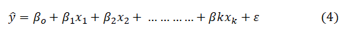
The collected data were analyzed by the linear regression method. This method estimates the effect of each independent variable (x) on the dependent variable (y). Therefore, the data were analyzed by drawing a linear regression line, a histogram, a residuals QQ-plot, a residuals x-plot and a distribution chart. We calculated the R-squared, the R and the outliers, then tested the fit of the linear model to the data and checked the residuals' normality assumption and the priori power. In general, the regression line equation provides the value of the predicted variable (Ŷ) by the following formula:

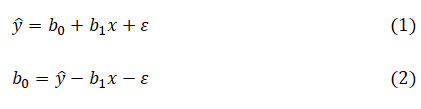
where b₀ is the y-intercept, where the line crosses the y-axis and b1 is the slope that describes the line's direction and inclination. In addition, ε is an aimless error component. Moreover, b₁ is connected with the data point by the following relation:

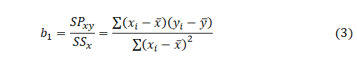
However, in the case of multiple linear regressions, the variant y may be related to k regressors and x₁, x₂……….x_k and Eq. 1 become as follows:

The confidence interval is the prediction interval of the mean value of the dependent variable, which has been calculated from the standard error of the confidence interval

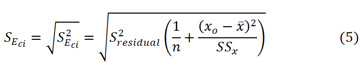
where the standard deviation of residual (S_residual) is calculated from the relation as

Therefore, the confidence interval (C_I) is calculated as

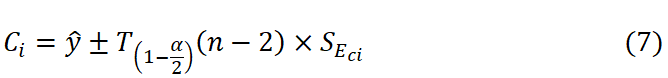
The prediction interval is an interval for a specific point value of the dependent variable that has been calculated from the standard error of the prediction interval

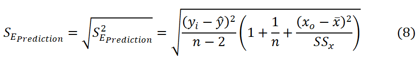
Therefore, the prediction interval (P_i) is calculated as

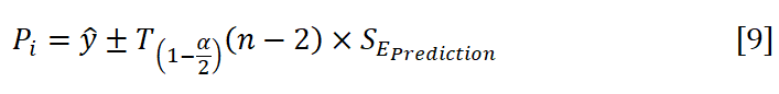
In addition to the above calculations, another parameter, identified as the percentage of the variance (R²), is explained by the regression (SSR_egression) from the overall variance (SS_Total) and followed by the equation

Algorithms

Here, we used the “R” programming language and linear regression algorithm. The language is as follows:

rm(list=ls())

if(! "car" %in% installed.packages()){install.packages("car")}

library(car)

x10 ≤ c(date ……………………….…..)

x11 ≤ c(date …………………………..)

x1 ≤ c(x10, x11)

y10 ≤ c(magnitude …………………..)

y11 ≤ c(magnitude ………………………..)

y1 ≤ c(y10, y11)

x0 ≤ c(2019, 2020, 2021, 2022, 2023, 2040, 2050)

model1=lm(y1~x1)

summary(model1)

predict(model1,data.frame(x1=x0),interval="confidence")

predict(model1,data.frame(x1=x0),interval="predict"

In addition, the steps of the algorithm for the linear regression process are as follows, and the information scheme is as follows:

Data-remapped

Lag_Magnitude-1

Lag_Magnitude-2

Lag_Magnitude-3

Lag_Magnitude-4

Lag_Magnitude-5

Lag_Magnitude-6

Lag_Magnitude-7

Lag_Magnitude-8

Lag_Magnitude-9

Lag_Magnitude-10

Lag_Magnitude-11

Lag_Magnitude-12

Data-remapped^2

Data-remapped^3

Date-remapped^*Lag_Magnitude-1

Data-remapped^*Lag_Magnitude-2

Data-remapped^*Lag_Magnitude-3

Data-remapped^*Lag_Magnitude-4

Data-remapped^*Lag_Magnitude-5

Date-remapped^*Lag_Magnitude-6

Data-remapped^*Lag_Magnitude-7

Data-remapped^*Lag_Magnitude-8

Data-remapped^*Lag_Magnitude-9

Data-remapped^*Lag_Magnitude-10

Date-remapped^*Lag_Magnitude-11

Data-remapped^*Lag_Magnitude-12

The magnitude was used in that algorithm as follows:

0.3654 × Lag_Magnitude-1+0.1332 × Lag_Magnitude-5+-0.3288 × Lag_Magnitude-6+0.3907 × Lag_Magnitude-7+-0.1579 × Lag_Magnitude-8+0.1527 × Lag_Magnitude-12+0 × Dateremapped^ 2+-0 × Date-remapped^3+-0.0012 × Date-remapped × Lag_Magnitude-1+0.0005 × Date-remapped × Lag_Magnitude-2 +0.0011 × Date-remapped × Lag_Magnitude-3+-0.0005 × Dateremapped × Lag_Magnitude-4+0.0023 × Date-remapped × Lag_Magnitude-6+-0.0025 × Date-remapped × Lag_Magnitude-7+0.0007 × Date-remapped × Lag_Magnitude-8+0.0006 × Dateremapped × Lag_Magnitude-11+-0.0021 × Date-remapped Finally, cross-validation was performed for statistical analysis.

Results and Discussion

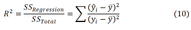
The analysis of the earthquake was performed based on two attributes, date and magnitude, which are related to each other. However, from the data, it is observed that the intensities of earthquakes in Bangladesh vary from very minor (≤ 2.8 Ms) to great (≥ 8.0 Ms) levels. Therefore, the percentage of these levels was calculated and is presented in Figure 5 (a) and most of the earthquakes were of light level (4.0 ≤ Ms<5.0). Moreover, the histogram of these intensities determines the average value of 4.6 ± 0.02 Ms from the Gaussian fitting of the frequency versus magnitude graph, as depicted in Figure 5(b). However, the data were trained and followed by the linear regression algorithm and then we obtained some new dates from which we could call the predicted dates. Figure 6 shows the statistical map of the earthquake magnitudes from 1933 to 2018 in Bangladesh and the data are trained considering the date to the x-axis and to obtain the magnitude from the y-axis using Weka explorer.

Here, the model and evaluation depend on the clustered instances extracted from the Weka software:

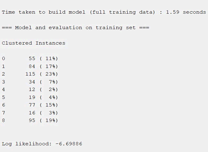
Figure 5: Data analysis of earthquakes that occurred from 1933 to 2018 in Bangladesh showing (a) Percentages of intensity and (b) Histogram of those intensities to determine the average value.

Figure 6: Visualization of the magnitude of earthquakes determined from 1933 to 2018 in Bangladesh. The data are trained considering the date to the x-axis and obtain the magnitude against it from the y-axis using the Weka explorer.

Therefore, a plot matrix of the earthquake data from 1933 to 2018 in Bangladesh has been achieved, as illustrated in Figures 7 and 8. The experiment was performed over 506 data points and the summary of observations is as follows:

Figure 7: Plot matrix of the earthquake data from 1918 to 2018 in Bangladesh and the data are trained by the linear regression method in Weka Explorer.

Figure 8: Analysis of earthquake data for Bangladesh between 2007 and 2018 showing (a) fitting by the linear regression method to correlates between real data and estimated data, (b)

As the data have already been trained, the final experiment for the prediction was established over the data points from 2007 to 2018 to achieve better fitting and closer prediction. Figure 8(a) displays the fitting by the linear regression method that correlates the real data to the estimated data points, resulting in a regression line with extrapolation. Therefore, the probable magnitude of the earthquake in the future will be on the extrapolated line. However, minor errors occur while the data mining process is performed, as illustrated in Figure 8(b). Here, the minor error is represented by the confidence interval and prediction interval, which are approximately 95%. In addition, Figure 8(c) displays the residual fitting data, which are controlled. Finally, the predicted variable (Ŷ) generates an equation, followed by Eq. 4 as

where b₁≈0.06 and α=(b_o+c)≈-115.84 along with the parameters R²≈0.046 and p<0.001. Table 2 represents the statistical data evaluated from the overall calculation and standard errors. From the analysis, it is observed that the value of R² is equal to ~0.046, which implies that 4.6% of the variability of y is explained by x and that the correlation is ~0.214. This means that there is a weak direct relationship between x and y. However, while the slope (b₁) is ~.06 and the confidence interval (C_I) is 0.03533141237 and 0.08431039783, y is increased by ~0.0598 for the increase in x by 1. Therefore, based on this statistical evaluation, the prediction of the earthquake has been performed over a few years approximately 2023 and estimated magnitudes that are included in Table 3. In addition, the comparison between the real data and the predicted data for these selected years is shown in Table 4. The regression line along with the prediction interval (P_i) and confidence interval (C_i) is depicted in Figure 9 (a) and 95% of p_i and C_i is observed in Figure 9(b). Moreover, the fitting parameter illustrated in Figure 10 (a) determines the accuracy of the analysis and the histogram of the residual lies between -0.5 and 0.5. Figure 10(b) displays the deviation of real data from the theoretical quantiles.

Table 2: Statistical mean values extracted from the linear regression method providing residual outliers (S_res), threshold outliers (k × S_res), standard error of confidence interval, Confidence Interval (C_I), standard error of the prediction interval, Prediction interval (P_i ) and percentage of the variance (R²).

Table 3: Statistical data for some selected years extracted from the linear regression method providing the predicted magnitude (Ŷ) of earthquakes in Bangladesh, and the statistical parameters are discussed above.

Table 4: A comparison with the real data of the magnitude of earthquakes in Bangladesh; the yellow highlights indicate the future predictions.

Figure 9: Prediction of magnitude of earthquake in Bangladesh based on previous year data showing (a) Extrapolation of regression line to the year of 2015 and (b) Confidence interval and prediction interval of 95%.

Figure 10: Fitting parameters obtained from the linear regression method showing (a) Histogram of the residual and (b) Deviation of real data from the theoretical quantiles.

Apart from this, the whole analysis has been implemented to develop a website so that people can be aware of earthquakes before the incident. The first page of the application is depicted in Figure 11. In this website, there is an option of selecting a time base to compare real data and predicted data and the earthquake zone can be selected, which was prepared from the regression analysis of longitude and latitude. In addition, a comparison between real and predicted data has been generated by this web application. Figures 12-14 display the predictions for 2016, 2017 and 2018, respectively. It is observed from the application that almost 70%-80% of the data are matched. However, the website can also detect the risk factors for the probable fault zones of earthquakes in Bangladesh, as illustrated in Figure 15. Therefore, a selection was performed for the region of Sunamganj (northeastern part of Bangladesh) and Figure 16 displays that the region is the most region located in the Sylhet fault zone.

Figure 11: Front page of the web application implementation.

Figure 12: Real data and predicted data comparison for the year 2016 evaluated by the web application.

Figure 13: Real data and predicted data comparison for the year 2017 evaluated by the web application.

Figure 14: Real data and predicted data comparison for the year 2018 evaluated by the web application.

Figure 15: Selection of the fault zone of earthquake evaluated by the web application.

Figure 16: Selection of the Sylhet fault zone of earthquake evaluated by the web application.

Conclusion

Earthquake prediction analysis has been performed for more than 100 years with conspicuous triumphs. The main obstacle to the prediction depends on the data extraction of precursory phenomena. Various computational methods and tools have been used for the detection of precursors by extracting normal information from large amounts of data. The mathematical analysis was performed by the linear regression method. In addition, the common framework of clustering explores the multiresolution analysis of seismic data starting from the raw data events described by their magnitude. A successful prediction with 70%-80% accuracy was achieved by this procedure. However, this new methodology may also be conducted for the analysis of data from geological phenomena, e.g., one can use this clustering method for volcanic eruptions.

Funding

The authors declare that no funds, grants or other support was received during the preparation of this manuscript.

Competing Interests

The authors have no relevant financial or nonfinancial interests to disclose.

Author Contributions

All authors contributed to the study conception and design. Material preparation, data collection and analysis were performed by Md. Imrul Kais, Md. Tanvir Islam Mim, Syed Sabit Hossain, Md. Sazzadur Ahamed, Ejaj Tarif and Md. Sarowar Hossain. The first draft of the manuscript was written by Md. Sarowar Hossain and all authors commented on previous versions of the manuscript. All the authors have read and approved the final manuscript. The authorship principles are referred below:

• Conception and design: Sarowar Hossain, Sazzadur Ahamed.
• Data collection: Imrul Kais, Syed Sabit Hossain.
• Formal analysis: Tanvir Islam Mim, Sarowar Hossain, and Ejaj Tarif.
• Investigation: Sarowar Hossain.
• Methodology: Imrul Kais and Sarowar Hossain.
• Project administration: Sazzadur Ahamed.
• Resources: Imrul Kais and Tanvir Islam Mim.
• Software: Imrul Kais, Tanvir Islam Mim and Sarowar Hossain.
• Supervision: Sarowar Hossain and Sazzadur Ahamed.
• Validation: Sarowar Hossain, Tanvir Islam Mim, Ejaj Tarif.
• Visualization: Sarowar Hossain, Ejaj Tarif, and Imrul Kais.
• Writing-original draft: Sarowar Hossain and Tanvir Islam Mim.
• Writing-review editing: Sarowar Hossain, Tanvir Islam Mim, Imrul Kais, and Ejaj Tarif.

References

1. Spence W, Sipkin SA, Choy GL. Measuring the size of an earthquake. Earthquake Inform Bullet (USGS). 1989;21(1):58-63.

   [Crossref]

2. Naddaf M. Turkey–Syria earthquake: What scientists know. Nature. 2023;614:398-399.

   [Crossref] [Google Scholar] [PubMed]

3. Kolbe AR, Hutson RA, Shannon H, Trzcinski E, Miles B, Levitz N, et al. Mortality, crime and access to basic needs before and after the Haiti earthquake: A random survey of Port-au-Prince households. Med Confl Surviv. 2010;26(4):281-297.

   [Crossref] [Google Scholar] [PubMed]

4. The Associated Press. Massive quake kills nearly 10,000 in China. NBC News. May 12. 2008.
5. Durrani AJ, Elnashai AS, Hashash Y, Kim SJ, Masud A. The Kashmir earthquake of October 8, 2005: A quick look report. MAE Center CD Release 05-04. 2005.

   [Google Scholar]

6. Kumar A, Gupta SC, Jindal AK, Jain S, Vandana. Aftershock activity of Bhuj earthquake of January 26th, 2001. J Earth Syst Sci. 2003;112:391–395.

   [Crossref] [Google Scholar]

7. The Associated Press. 15 years of Gujarat earthquake: A trauma etched in Gujarat's memory, The Times of India, January 26. 2007.
8. Adhikari LB, Gautam UP, Koirala BP, Bhattarai M, Kandel T, Gupta RM, et al. The aftershock sequence of the 2015 April 25 Gorkha-Nepal earthquake. Geophys J Int. 2015;203(3):2119-2124.

   [Crossref] [Google Scholar]

9. Rechard Pallardy Qinghai earthquake of 2010, Britannica, August 13. 2010.
10. Yeats RS, Madden C. Damage from the Nahrin, Afghanistan, Earthquake of 25 March 2002. Seismol Res Lett. 2003;74(3):305-311.

    [Crossref] [Google Scholar]

11. Sands L, Cursino M. Afghan earthquake: At least 1,000 people killed and 1,500 injured, BBC News, June 22. 2022.
12. Raihanul I, Nazrul MI. Earthquake risks in Bangladesh: Causes, vulnerability, preparedness and strategies for mitigation. ARPN J Earth Sci. 2016;5(2):75-90.
13. Roy S. Probabilistic prediction for earthquake in Bangladesh: Just How big does the earthquake have to be next years? Open J Earthquake Res. 2014;3:108-114.

    [Google Scholar]

14. Apu N, Urmi Das. Tectonics and earthquake potential of Bangladesh: A review. Int J Disast Resilience Built Environ. 2020;12(3):295-307.

    [Crossref] [Google Scholar]

15. Islam AS, Ahmad SI, Jumaat MZ, Hussain RR, Rahman MA, Darain KM. Efficient design in building construction with rubber bearing in medium risk seismicity: Case study and assessment. J Civ Eng Manag. 2014;20(5):621-631.

    [Crossref] [Google Scholar]

16. Prakash K, Yuan X, Ravi K, Rainer K, Chadha RK. The rapid drift of the Indian tectonic plate. Nature. 2007;449:894-897.
17. Lauren H. Rock magnetism uncrumples the Himalayas’ complex collision zone, MIT News, January 7. 2021.
18. Rashied M, Mahmud A. Potential amplifiable areas in Dhaka city for seismic hazard. J Bangladesh Inst Plan. 2019;12:33-43.

    [Google Scholar]

19. Abdullah M, Nusrath J. A study of earthquakes in Bangladesh and the data analysis of the earthquakes that were generated in Bangladesh and its’ very close regions for the last forty years (1976-2016). J Geol Geophys. 2017;6(4):1-5.

    [Google Scholar]

20. Zaman M, Rakhine S. Earthquake risks in Bangladesh and evaluation of awareness among the university students. J Earth Sci Clim Change. 2018;9(7):1-7.