Advances in Automobile Engineering
Open Access
ISSN: 2167-7670
ISSN: 2167-7670
Research Article - (2016) Volume 5, Issue 2
No.2918 Turkish Highway Traffic Act has been the reference legislation for traffic accidents in Turkey since 1983. Although this act consists of several explanations and definitions, it has still deficiencies especially in defining fault rates which are vital for traffic accident analyses. Accident experts determine fault rates mostly according to their initiatives without conducting scientific analyses on accidents due to inadequate quantitative instructions on fault rates in the act. Speed analyses of accident involvements play an important role in accident investigations. A more comprehensive parameter, Energy Equivalent Speed, may be defined to explain dissipation and severity of deformation energy and crush amounts formed on vehicles which also give hint about fault rates. In this study, accessible data were collected from a sample accident scene (police reports, skid marks, deformation situations, crush depths etc.) and used as inputs for an accident reconstruction software called “vCrash” which is able to simulate the accident scene in 2D and 3D. Energy equivalent speed calculations were achieved using 784 parameters with a prediction error. Multi-layer Feed Forward Neural Network and Generalized Regression Neural Network models were utilized for estimation of energy equivalent speeds (speeds just before the collision, i.e., in case of absence of skid marks) based on using these parameters as teaching data for the models. It was aimed that, by benefiting from these neural network methods, necessity of using expensive simulation softwares for probable accidents in future may be avoided. In order to observe performance of the neural network models, standard error of estimates (mean square error) and multiple correlation coefficients were also analyzed using 5-fold cross validation on the dataset. It was observed that, in general, Multi-layer Feed Forward Neural Network model yielded better results for both energy equivalent speed and fault rate analyses. Based on simulation results (energy equivalent speeds and deformations) and assumption of a fault rate scale, fault rates were estimated on prediction models by assuming correspondence of every predetermined increment in energy equivalent speed of specific involvement to a specific increment in fault rate of the same involvement to put forward a scientific and systematic approach and compensate deficiencies in the act.
<Keywords: Accident reconstruction; Fault rate; Energy equivalent speed; Prediction models
Transportation engineering firstly focuses on safety and efficiency. Public agencies put forward substantial efforts on reducing traffic accidents which also entails a huge financial burden on society. Occurrence of traffic accidents strictly depends on two major factors: driver and roadway design. Gender and age of the driver are of great importance in traffic [1]. Death rates usually tend to fall as countries develop. However, fatalities in traffic accidents grow proportionally to development of a country which means that increment in the number of motor vehicles usually brings an increase in road traffic accidents.
Injuries in traffic accidents are the primary reason of injury related deaths all around the world. April 7 was devoted to prevention of traffic injuries by World Health Organization (WHO) in 2004. As in many countries, in Turkey, fatalities and injuries due to traffic accidents are major problems for public [2]. Reckless driving with excessive speed gives rise to most of the traffic accidents [3]. According to WHO, traffic fatalities will be the sixth leading cause of death worldwide by the year 2020 [4].
According to 2002 annual reports, traffic accidents are the 11th reason for fatalities in Turkey. Traffic accidents have the 2nd priority for fatalities at the age interval of 5-29 and the 3rd for the age interval of 30-44. In 1999, while the number of registered traffic accidents was 466000, it was 501000 in year 2000. General Directorate of Highway reports indicates 2954 fatalities and 94497 injuries involving 409407 accidents in the year 2001 and 570419 accidents in the year 2005 [5].
In the software step; simulation of a sample property damage only (PDO) accident (one of the most frequent in Turkey) was conducted on vCrash [6]. Referring to energy transfer and impulse-momentum analysis results of the software; formation of the accident, location of vehicle after the collision damages comprised on the collision regions were examined. In the following step, Energy Equivalent Speed (EES) values (or speed values) which were also directly proportional to deformations formed on the collision regions and fault rates were calculated by benefiting from 784 parameters (used for crash simulation) as teaching data for Multi-layer Feed Forward Neural Network (MFFNN) and Generalized Regression Neural Network (GRNN) models. After training the models in terms of every EES corresponding to every deformation (crush depth), predicted EES values and deformations were used as input data for the models to estimate fault rates as output data. Referring to this method, experts may refrain from using expensive reconstruction softwares for accident analysis in future.
Analysis of the sample accident scenario
In the sample accident case, two average passenger cars (APC) collide with each other at an angle of 90° on an equal-arm intersection (no traffic lights, “STOP”, “YIELD”, etc. warning signs and/or officer) as shown in Figure 1.

Figure 1: First contact moment of vehicles on the software.
Referring to No.2918 Turkish Highway Traffic Act (THTA), in such cases vehicle 1 (right) has the passing priority rather than vehicle 2 (left). For this kind of situations, it is assumed by the experts that the vehicle 2 is at-fault and vehicle 1 is deemed as minor faulty due to careless aggressing to the intersection. The fault rates are generally allocated to 75%-25% or 80%-20% by initiative of experts. However, several questions arise about collision speeds, absence/existence of skid marks on the road surface, intersection approaching speed of vehicle 1 (if above legal speed limits, is he/she still minor-faulty?), existence of a systematic method for fault rate determination.
Collision speeds are directly proportional to EES which directly defines the relation between contact speed and deformation on vehicles [7]. In other words, it is the measure of collision speed which transforms into deformation. In case of absence of skid marks (mostly anti-lock braking system equipped vehicles), the biggest clue about the speeds of vehicles was the damage formed on the vehicles. More damage on the vehicle(s), more energy transformed into deformation energy which is defined as crush depth (Sdef) in terms of meters. For the first scenario, vehicles were crashed into each other at angle of 90º with estimated initial speeds and deformation amounts were recorded. Coefficient of friction (μ) on road surface was assumed as 1 (fully dry surface). EES values from simulation and parameters for training MFFNN and GRNN for EES prediction are:
Pre-impact velocity (ν1): Velocity of vehicle(s) at the time of contact to each other, km/h.
Post-impact velocity (ν2): Velocity of vehicle(s) at the time of separation from each other, km/h.
Deformation (ε): Average crush depth of damaged region, m
Pre-omega and post-omega (ω1, ω2): Angular velocities of vehicles at the time of contact to each other and at the time of separation from each other, respectively, rad/s.
Impulse (Imp): The result of impact force, over a specific time period “t”, N.s.
Time (t): Time elapsed during the collision in seconds (s).
x, y, z: Location of involvements just before the collision in Cartesian coordinates, m.
Delta-v (Δv): The change in velocity of a vehicle’s occupant compartment during the collision phase of a motor vehicle crash (i.e.,from the moment of initial contact between vehicles until the moment of their separation), km/h [7].
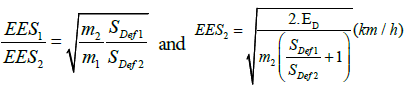
Energy Equivalent Speed (EES): EES has been defined by Burg, Martin and Zeidler in the year 1980 and was suggested for a common use. EES is a speed measure which will be transformed into deformation energy during the collision or in international standard definition, “The equivalent speed at which a particular vehicle would need to contact any fixed rigid object in order to dissipate the deformation energy corresponding to the observed vehicle residual crush.” The kinetic energy of the vehicle with virtual velocity “EES” defines the plastic deformation (damage) formed on the vehicle. Energy absorption depends on various parameters. Thus, several crash tests under different conditions must be done to determine EES accurately. If the EES of one vehicle is known, then it is possible to determine the unknown EES based on the principle of action equals reaction by approximating the other crush. EES may be calculated as shown in Eq. (1).
 (1)
(1)
where,
m1, m2: mass of each vehicle, kg
sDef1, sDef2: crush depth of each vehicle, outer surface to impact point in line with impact force, m ED: energy lost by both vehicles in the collision due to damage, J.
A compression phase followed by a restitution phase is comprised during a collision. The compression phase lasts from the contact of the vehicle with an obstacle (another vehicle or anything else) to the point of maximum compression. During this phase, the energy is stocked until the maximum deformation. The restitution phase begins when deformation is maximum and ends when the vehicle separates from the obstacle. During this phase, the deformation energy is released [7].
EES values of veh.1 and veh.2 were 19.03 km/h and 19.24 km/h, respectively, at the instant of collision (90o collision angle) assuming their collision speed as 20 km/h for each. According to expert report of this accident (expert initiative, absence of speed and deformation analyses), the fault rate of veh.2 is 80 and the others’ is 20, out of 100.
Deformation Energy (E): Plastic deformation affiliated to the kinetic energy of the vehicle with virtual velocity “EES”, J.
Generalized extreme value (GEV): Possible limit distribution of properly normalized maxima of a sequence of independent and identically distributed random variables [8].
Prediction methods
Multi-layer Feed-Forward Neural Network (MFFNN): Input, output and hidden layers form an MFNN model (Figure 2). Weighted inputs are received from a previous layer and their outputs are transmitted to next-layer neurons. A nonlinear activation function is used to transfer the summations of weighted input signals. In order to conduct an error analysis, a comparison with actual results is made until the error reaches an acceptable value [9].
In Figure 2, Xi: neuron input, Wij, Wkj: weights, M: number of neurons in the hidden layer, Y: output value [10].

Figure 2: MFFNN architecture.
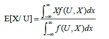
Generalized Regression Neural Networks (GRNN): In GRNN, linear and nonlinear regression can be performed by generalization of both radial basis function networks and probabilistic neural networks [11]. Basis function architectures are used to approximate any arbitrary function between input and output vectors directly from training samples along with their usage for multidimensional interpolation [9-14]. Estimation of a linear or nonlinear regression surface on independent variables (input vectors) “U” and dependent variables (desired output vectors) “X” is the main function of GRNN. In other saying, just by training “U”, the most probable value of an output, Ox, is computed by the network. Particularly, the computation of the joint probability density function of U and X is conducted by the network. The expected value of X given U is expressed as [11]:
 (2)
(2)
EES prediction
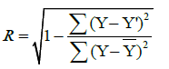
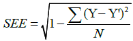
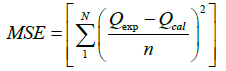
The dataset used for EES prediction contains 14 predictor variables (t, x-y-z, phi, Δv, Imp, E, ε, ν1, ν2, ω1, ω2, GEV). Descriptive statistics for the dataset is given in Table 1. The performance of both models were evaluated by using 5-fold cross validation and calculating the standard error of estimates (SEE) and multiple coefficient of regression (R), whose formulas are given in Eqs. (3) and (4), respectively.
 (3)
(3)
 (4)
(4)
| Statistics Name | ||||
|---|---|---|---|---|
| Data | Mean | Maximum | Minimum | Std. Deviation |
| t | 1,662 | 5,623 | 0,06 | 1,174 |
| x | 8,525 | 111,657 | -78,109 | 30,132 |
| y | -1,436 | 8,756 | -80,962 | 16,494 |
| z | 0,431 | 0,642 | 0,005 | 0,114 |
| phi | 86,912 | 169,632 | 0,066 | 45,521 |
| Δv1 | 8,771 | 75,095 | 0,237 | 14,759 |
| Imp | 10,232,695 | 100,421,035 | 532,244 | 19,552,068 |
| E | 74,885,498 | 1,112,047,522 | 781,718 | 203,235,981 |
| ε | 0,200 | 0,705 | 0,025 | 0,142 |
| ν1 | 28,290 | 90,471 | 0 | 25,613 |
| ω1 | 0,053 | 1,724 | -0,487 | 0,270 |
| ν2 | 25,234 | 69,384 | 0,055 | 19,391 |
| ω2 | 0,245 | 8,085 | -3,708 | 1,597 |
| Δv2 | 14,814 | 48,092 | 0 | 12,620 |
| GEV | 0,988 | 1,614 | 0 | 0,388 |
| EES | 14,521 | 44,215 | 0,002 | 10,938 |
Table 1: Dataset statistics.
In (3) and (4), Y corresponds to measured EES value, Y’ corresponds to predicted EES value, Y is the mean of the measured values of EES and N is the number of samples in a test subset.
Principal Component Analysis is used to orthogonalize the components of the input vectors by pre-processing them (so that they are uncorrelated with each other) and to sort the resulting orthogonal components (principal components) ensuring the first order of the largest variation [12]. Default momentum values, number of epochs (selected as 100) and the learning rate are the other important parameters within the model [13].
For both MFFNN-based and GRNN-based EES prediction models, the individual SEE and R values for each fold as well as their average are shown in Table 2. The averages are simply the arithmetic averages of the SEE and R values of each fold. As it is clearly seen from Table 2, the GRNN-based model gave higher averaged R and SEE values for EES prediction and both were lower for MFFNN-based model.
| MFFNN-based | GRNN-based | |||||
|---|---|---|---|---|---|---|
| model | model | |||||
| Folds | R | SEE | R | SEE | ||
| Fold 1 | 0,86 | 3,32 | 0,93 | 3,69 | ||
| Fold 2 | 0,87 | 3,63 | 0,88 | 4,55 | ||
| Fold 3 | 0,90 | 3,51 | 0,87 | 3,71 | ||
| Fold 4 | 0,83 | 4,43 | 0,89 | 4,41 | ||
| Fold 5 | 0,93 | 2,19 | 0,91 | 4,75 | ||
| Average | 0,88 | 3,42 | 0,90 | 4,22 | ||
Table 2: R and SEE values of the MFFNN and GRNN models by means of 5-fold cross-validation (EES prediction).
Fault rate prediction
In the software step of this study, similar vehicles with ones in real world accident were crashed into each other by varying their speeds (EES) within every simulation related to the scenario. Every speed change corresponded to varied deformation amounts on collision regions of the involvements. While one of the involvement’s speeds was kept constant, the others’ was increased by 5 km/h within each simulation. It was assumed that every 5 km/h increment in speed of involvements corresponded to 3 points increment in fault rates of the related vehicle. Every increment in speeds means proportional increment in EES values. Every deformation (Sdef) related to every speed value was taken from the report by repeating the simulation. One of the speed values was kept constant and the other was changed for every 20 trials until 500 data were obtained for the accident scenario. Table 3 depicts the statistics of the deformations, speeds and fault rates.
| Deformation (m) (veh.1) | Deformation (m) (veh.2) | Speed (EES) (km/h) (veh.1) | Speed (EES) (km/h) (veh.2) | Fault Rate (%) (veh.1) | Fault Rate (%) (veh.2) | |
|---|---|---|---|---|---|---|
| Minimum | 0.072 | 0.065 | 15 | 20 | 0 | 18 |
| Maximum | 1.637 | 1.598 | 170 | 175 | 82 | 100 |
| Mean | 0.849 | 0.774 | 68.818 | 74.108 | 28.028 | 72 |
| Std. Dev. | 0.421 | 0.408 | 37.198 | 36.672 | 26.786 | 26.797 |
Table 3: Descriptive statistics for the scenario.
MFFNN and GRNN models were comprised and adopted separately to the dataset. Prediction of fault rates within these models was achieved by using SDef1, SDef2, V1 (predicted EES1) and V2 (predicted EES2) as input variables and Fault-rate1 and Fault-rate2 as output variables.
The input, hidden and output layers of MFFNN have 4, 20 and 2 neurons, respectively (Figure 3). An activation function of tan-sigmoid in the hidden layer and a pure-linear activation function in the output layer were used where Levenberg–Marquardt algorithm was utilized for training the network. The number of epochs, the learning rate and momentum were selected as 500, 0.03 and 0.4, respectively.

Figure 3: rM faFuFltrNaNte mpreoddiectli ofonr. faultrate prediction.
Spread constant has a drastic effect on prediction performance. It should be noted that since the most important architectural parameter of GRNN model is the spread constant, which has certain effect on prediction efficiency. In this paper, the spread value was set to 2.5 (default 1.0) empirically.
Within developing the models, each input and output variables of 500 simulations were used. The data was randomly divided into two disjoint subsets using 5-fold cross validation. The training set had 400 observations and testing set 100. Mean squared error (MSE) in Eq. (5) and R in Eq. (6) were utilized in order to compare the prediction ability of the developed models. MATLAB software [15] was used for performing the experiments.
 (5)
(5)
and 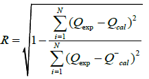 (6)
(6)
where;
Qexp: observed value; Qcal: predicted value
Qexp: mean predicted value; N: number of data points
Fault rate prediction performance of models is demonstrated in Table 4.
| MSE | R | |||
|---|---|---|---|---|
| Fold Number | MFFNN | GRNN | MFFNN | GRNN |
| 1 | 1.01111 | 2.512337 | 0.999492 | 0.997346 |
| 2 | 1.016606 | 3.517386 | 0.999598 | 0.994529 |
| 3 | 2.100327 | 3.800502 | 0.99919 | 0.993723 |
| 4 | 4.081504 | 4.292495 | 0.998548 | 0.991565 |
| 5 | 0.705644 | 2.934098 | 0.999708 | 0.995829 |
| Average | 1.783038 | 3.411364 | 0.999307 | 0.994598 |
Table 4: Results of the scenario by means of 5-fold cross-validation (Fault rate prediction).
The followings can be concluded from Tables 2 and 4:
In average, MFFNN model performed better results (i.e., higher R and lower MSE) than GRNN prediction model in terms of fault rate prediction.
For EES prediction, MFFNN gave lower MSE and R values whereas GRNN gave higher for both.
Absence of training phase in GRNN yielded much faster result production than MFFNN.
Acceptable R values were achieved for prediction of fault rates for all folds and scenarios (all were close to 1).
At this term, a sample traffic accident was examined with the aid of data collection from the accident scene. Simulation and analysis relevant to these data were conducted on traffic accident reconstruction tool (software) called vCrash which showed damage levels comprised on involvements, EES values and other 14 parameters in 3D. As a result, these examinations were interpreted to comprehend the general reasons causing these accidents and precautions to minimize them. MFFNN and GRNN models were used to develop new models for EES prediction by using vCrash variables. According to results of EES and fault rate prediction, MFFNN and GRNN models may be valid predictors also for avoiding necessity of using expensive simulation softwares for probable accidents in future in order to help prediction of fault rates impartially, scientifically and systematically.
This study aims at bringing a new aspect and scientific approach for examination and determination fault rates in most frequent accidents in Turkey. It focuses on fulfilling the needs by implying some deficiencies in THTA and eliminating initiative and/or experience of experts. Direct proportion between collision speed and deformation is the key matter for bringing these kinds of issues to light. Thanks to vCrash software, the accident scene was simulated followed by the second stage of the study in which the dataset was obtained (i.e., deformation energy, EES, fault rate) of the accident scene. MFFNN and GRNN prediction models were comprised to predict fault rates in which R and MSE values and performance of the models was also investigated. The performance of MFFNN was better on fault rate prediction than GRNN (lower MSE, higher R) except R in EES prediction. In average, MFFNN gave more accurate results than GRNN, but GRNN was the fastest in prediction process. These algorithms may be used with an interface (application) that can run on a portable device (cell phone, tablet, etc.) which can also be used to predict the fault rates at the accident scene just by entering average deformations formed on the collision regions. Besides, this approach may also help fair decisions to be made in courts and forensic investigations. Currently in Turkey, insurance companies just consider 100%, 50% and 0% fault rate situations in case of an accident. Thus, this study may also be useful for finer fault rate determination. Besides, these algorithms are more likely suitable applications to commercialize.
This study was supported by Cukurova University, Scientific Research Project (FDK-2014-2863).