Journal of Geology & Geophysics
Open Access
ISSN: 2381-8719
ISSN: 2381-8719
Research Article - (2016) Volume 5, Issue 3
Deconvolution analysis of reflectance spectra has been a useful method to infer mineral composition and crystal structure. Many of the recent deconvolution analyses of reflectance spectra of major rock-forming minerals, such as olivine and pyroxene, have been based on a modified Gaussian Model (MGM). The numerical algorithm of the widely used MGM, however, utilizes the steepest descent method, which has a local minima problem. With inaccurate initial parameters, the steepest descent method converges into a local minimum, thus the analyzer must manually adjust initial parameters and calculate the model repeatedly to obtain the desired solution. In order to avoid the local minimum problem, we utilized Bayesian spectral deconvolution with the exchange Monte Carlo method, which is an improved algorithm of the Markov chain Monte Carlo method, aimed to both avoid local minima traps and remove the arbitrariness originated from initial parameters. We applied the model to visible to near infrared reflectance spectra of 31 synthetic clinopyroxene samples with wide ranging Mg, Fe and Ca compositions (solid solution). We obtained results consistent with the previous studies based on conventional MGM analyses, suggesting that the exchange Monte Carlo method can yield results consistent with the conventional MGM analyses purely based on the observed data. We also find that the center wavelengths of 1 μm absorption bands of high-Ca pyroxene samples have a linear dependence on Fe/Mg component. Both 1 μm and 2 μm absorption bands seem to follow approximation lines in the three-dimensional spaces of center wavelengths, Ca and Fe components. The successful application of the exchange Monte Carlo method to a wide range of clinopyroxenes would have a potential to expand the applicability of MGM to a variety of space/ground-based observations, especially when we cannot rely on prior information of the mineralogy.
Keywords: Pyroxene, Synthetic mineral, Reflection spectroscopy, Spectral deconvolution, Modified Gaussian model, Monte Carlo method
Remote sensing of reflectance spectra of Earth and other planetary bodies can be useful for identifying mineral distribution on their surfaces, especially in remote regions that are exceedingly challenging to perform field-based investigation, and those planetary surfaces yet to have in situ observation, mapping, characterization, sampling, and analyses [1-8]. Many different factors, however, can influence the surface spectra, such as various alteration and weathering processes, and observational conditions [2,3,5,9-12]. Because a reflectance spectrum is a complex non-linear mixture of the above mentioned factors [13-16], it is highly challenging to segregate each factor and extract the true mineral spectra, based solely on remotely observed reflectance spectra, and thus confidence in the resulting signatures should be gained by comparing with the reference spectra obtained by field or laboratory measurements [17]. Though challenging, investigating the spectral change due to the variation of elemental composition should not be avoided, since it is one of the ultimate goals of remote sensing of reflectance spectra of planetary surfaces [2,18]. Compared to terrestrial surfaces, those of extraterrestrial bodies such as the Moon and asteroids are not covered by liquid water and vegetation, and have negligible to no atmosphere, and thus may be considered to be the best places to observe the true nature of mineral spectra [19-25]. Yet, there are many factors to contaminate reflectance spectra of such planetary surfaces such as regolith particles, space weathering, and horizontal and vertical mixing by impact cratering, thus identifying the variation of mineral distribution on extraterrestrial bodies is still difficult [10,22,26-30]. Therefore, studying the spectral change using simple pure minerals that compose Earth and planetary surfaces is a critical foundational step to analyze reflectance spectra and is a prerequisite of reflectance spectroscopy, in light of continued application to planetary surfaces [8,31-35].
Deconvolution of reflectance spectra has been a common procedure for interpreting the experimental data of minerals and observation data of terrestrial and extraterrestrial surfaces. Among the most recognized spectral deconvolution methods in planetary science is the modified Gaussian model (MGM) [36,37]. In their paper, Sunshine et al. [36] showed that for 1 μm absorption band of orthopyroxene, Gaussian functions in the wavelength space fit better than Gaussians in the frequency space. The MGM express reflectance spectrum by the following function:
where R is reflectance, x is wavelength, and sk, μk and σk are the strength (amplitude), center (mean) and width (standard deviation) for kth Gaussian function, respectively. K is the number of Gaussian functions. The function C(x) is continuum of reflectance spectra:
where C0 and C1 are respectively intercept and slope of the continuum in frequency space.
The technical difficulty of applying the modified Gaussian model (MGM) is due to a local minima problem. The numerical algorithm of the widely used MGM utilizes the steepest descent method [36,38] or total inversion algorithm [37,39], both of which are not guaranteed to converge into a global solution. The analyzer can find an optimal solution only when the appropriate initial parameters are provided, based on preliminary knowledge of mineralogy [40,41]. With inaccurate initial parameters, however, these gradient descent methods converge into local minima, and thus the analyzer must manually adjust initial parameters and calculate the model iteratively to obtain the desired solution [16,42]. This would be a significant obstacle when one needs to automatically analyze large spectral databases obtained by space missions. In addition, preliminary knowledge of mineralogy may not always be available for space/ground-based observations, especially when the reflectance spectra are the only useful obtained data for interpreting the mineralogy of target bodies. Given the recent rapid increase of reflectance spectral data, automation of deconvolution analysis without requiring preliminary information on mineralogy is warranted. Makarewicz et al. [43] and Parente et al. [42] recently developed an algorithm to select initial band parameters automatically, based on inflection points of the derivatives of observed spectra. Although their algorithm does not depend on prior information, many spurious local minima and inflection points due to noise lead the authors to apply a smoothing filter, yielding arbitrariness on their analyses.
In order to overcome the local minima problem, the exchange Monte Carlo method, also known as parallel tempering [44], has been widely applied in the fields of physics, chemistry, biology, engineering and materials science [45]. Nagata et al. [46] developed a Bayesian spectral deconvolution model combined with the exchange Monte Carlo method with application to visible to near-infrared (Vis/NIR) reflectance spectra of fayalite and forsterite. This method is an improved algorithm of the Markov chain Monte Carlo method, aimed to avoid local minima traps [47] and to remove the arbitrariness originated from initial parameters. In order to solve the local minima problem, the simulated annealing scheme [48] has been incorporated into the model of Nagata et al. [46]. This algorithm introduces a pseudo-temperature and attempts to find the global minimum by heating and cooling the system. Nagata et al. [46] showed that the method can deconvolve reflectance spectral data of fayalite and forsterite into a few Gaussians with a continuum, purely based on the observed data, without requiring preliminary information of the band structure of olivine absorptions. In this paper, we report the applicability of the exchange Monte Carlo method to more complex rock-forming minerals (i.e., clinopyroxene). As described below, since the behavior of pyroxene spectra with the change of chemical composition is relatively well understood, the use of reflectance spectra of pyroxene minerals is suitable for testing the new spectral deconvolution method. Clinopyroxene (Cpx), with its general formula being (M2)(M1) (SiAl)2O6, is one of the most important rock-forming mineral groups due to both its rich abundance on solid bodies in the solar system and distinguished absorption features [20,34,49]. Cpx includes a wide range solid solution of Mg, Fe and Ca compositions and has two crystal structures of C2/c and P21/c [50], which could reflect various physical and chemical processes inside planetary bodies, such as the thermal history of magma [51]. Due to its wide range of chemical compositions, reflectance spectra of Cpx minerals vary significantly, and are generally grouped into three types: type-A, B and A/B [20,52,53]. Three major absorption bands are observed in type-B spectra, centered around 1.0, 1.2, and 2 μm, attributed to spin-allowed crystal field transitions of Fe cations in the octahedral (M1 and M2) sites [20]. These band centers are known to vary due to total iron and calcium content [19,52-55]. On the other hand, type-A spectra lack a strong 2 μm band, interpreted as a low Fe2+ content in the M2 site [53]. Type-A/B spectra are intermediate between type-A and B, although the boundaries are not well defined. MGM analyses have been performed to natural Cpx [36,53], synthetic Cpx [56], and mixtures of orthopyroxene-clinopyroxene [37,41].
Exchange Monte Carlo method
The technical details of the exchange Monte Carlo method is described elsewhere [46], thus we briefly summarize the key parameters of the model. In our study, the hyperparameters for Gamma and Gauss distributions used to yield probability densities of the parameters are those identified in Nagata et al. [46]: ηa = 3.0, λa = 2.0, ν0 = 1.25, ξ0 = 2.5, ηb = 5.0 and λb = 0.04. The total number of temperatures L in our study was 80, and the inverse temperature βl given by:
Figure 1 shows typical examples of the evolution of root mean square (RMS) during the exchange Monte Carlo calculations for sample 088 using 4 Gaussian functions. Rapid decreases of RMS for the lowest temperature can be observed at about Monte Carlo steps = 300, 500, 700, 1500, and 6000, due to the parameter exchange between the lowest and middle temperatures. From Figure 1, it can be observed that the RMSs of higher temperatures are generally larger than those of lower temperatures, showing attempts to find better global minimum with wider fluctuations. On the other hand, for lower temperatures, each iteration attempts to find local minimum within a parameter range narrower than higher temperatures. After the Monte Carlo step exceeds 104, although the model still attempts to find better solution with certain fluctuations of parameters, the RMSs remain almost constant, and the expectation values of parameters converge to the best solution. Similar to Nagata et al. [46], the Monte Carlo calculation was iterated through 100,000 steps for the burn-in period and 20,000 steps for the expectation value calculations. Errors of band parameters are estimated from 2σ based on ten runs using a different series of random numbers.
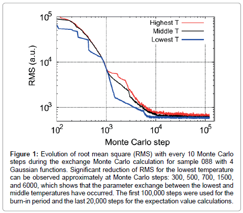
Figure 1: Evolution of root mean square (RMS) with every 10 Monte Carlo steps during the exchange Monte Carlo calculation for sample 088 with 4 Gaussian functions. Significant reduction of RMS for the lowest temperature can be observed approximately at Monte Carlo steps: 300, 500, 700, 1500, and 6000, which shows that the parameter exchange between the lowest and middle temperatures have occurred. The first 100,000 steps were used for the burn-in period and the last 20,000 steps for the expectation value calculations.
The number of Gaussian functions, K, is an important parameter for deconvolution analysis. The model usually improves with more Gaussians. Though, too many Gaussians may cause overfitting, and the solution can be physically unrealistic. We performed spectral deconvolution using a various number of Gaussian functions. For one spectrum, we varied K from 3 to 10, thus the total number of free parameters ranges from 11 to 32, including the intercept and slope of the continuum. In order to select an optimal K for the deconvolution, we calculate the free energy, or stochastic complexity [57,58], which is an evaluation function for the model section problem [46]. With increasing K, we find that the free energy decreases, and when K is higher than about 5, it converges and fluctuates around a low value. Thus, we chose minimum Ks from the region where the free energies converge and interpret them as optimal Ks, listed in Table 1.
| Compositionb | 1 µm band | 1.2 µm band | ||||||||
| SampleID | Minerala | En | Fs | Wo | Center (µm) | FWHM (µm) | Strength | Center (µm) | FWHM (µm) | Strength |
| 9 | Pigeonite | 43 | 47 | 10 | 0.956 ±0.0014 | 0.223 ± 0.004 | -1.32± 0.03 | 1.229 ± 0.008 | 0.30 ± 0.03 | -0.24 ± 0.03 |
| 11 | Pigeonite | 36 | 50 | 14 | 0.9579 ±0.0003 | 0.2342 ± 0.0007 | -2.040 ± 0.004 | 1.243 ± 0.0011 | 0.230 ± 0.003 | -0.416 ± 0.0013 |
| 53 | Pigeonite | 23 | 70 | 8 | 0.9646 ± 0.0003 | 0.233 ± 0.0011 | -2.042 ±0.004 | 1.258 ± 0.0013 | 0.244 ± 0.003 | -0.458 ± 0.005 |
| 88 | Pigeonite | 0 | 90 | 10 | 0.9801 ± 0.0004 | 0.2114 ± 0.0007 | -1.334 ± 0.003 | 1.245 ± 0.002 | 0.351 ± 0.003 | -0.3592± 0.0008 |
| 50 | Augite | 19 | 58 | 23 | 0.9808 ± 0.0003 | 0.235 ± 0.0013 | -2.307 ± 0.007 | 1.278 ± 0.002 | 0.265 ± 0.003 | -0.510 ± 0.005 |
| 51 | Augite | 39 | 34 | 27 | 0.991 ± 0.002 | 0.20 ± 0.010 | -1.6 ± 0.11 | 1.26 ± 0.014 | 0.34 ± 0.07 | -0.35 ± 0.08 |
| 54 | Augite | 6 | 70 | 23 | 0.988 ± 0.0013 | 0.250 ± 0.008 | -2.50 ± 0.02 | 1.290 ± 0.007 | 0.30 ± 0.010 | -0.70 ± 0.02 |
| 55 | Augite | 18 | 56 | 26 | 0.998 ±0.002 | 0.201 ± 0.005 | -1.9 ± 0.12 | 1.261 ± 0.003 | 0.331 ± 0.005 | -0.475 ± 0.008 |
| 56 | Augite | 18 | 60 | 22 | 0.9715 ±0.0004 | 0.241 ± 0.002 | -1.32 ± 0.014 | 1.260 ± 0.002 | 0.257 ± 0.006 | -0.32 ± 0.011 |
| 57 | Augite | 36 | 39 | 25 | 0.9915 ± 0.0004 | 0.1998 ± 0.0008 | -1.414 ± 0.004 | 1.269 ± 0.004 | 0.28 ± 0.02 | -0.182 ± 0.005 |
| 58 | Augite | 28 | 45 | 27 | 1.001 ± 0.004 | 0.198 ± 0.007 | -1.3 ± 0.14 | 1.26 ± 0.011 | 0.28± 0.02 | -0.29 ± 0.03 |
| 66 | Augite | 15 | 48 | 38 | 1.0128 ± 0.0003 | 0.1804 ± 0.0005 | -1.43 ± 0.02 | 1.227 ± 0.004 | 0.386 ± 0.009 | -0.443± 0.009 |
| 67 | Augite | 52 | 9 | 39 | 1.016 ±0.003 | 0.17 ± 0.011 | -1.0 ± 0.14 | 1.3 ± 0.13 | 0.3 ± 0.2 | -0.2 ± 0.10 |
| 68 | Augite | 29 | 33 | 38 | 1.008 ± 0.006 | 0.20 ± 0.011 | -1.8 ± 0.3 | 1.26 ± 0.010 | 0.33 ± 0.014 | -0.38 ± 0.012 |
| 73 | Augite | 36 | 25 | 39 | 1.0099 ±0.0003 | 0.163 ± 0.0010 | -1.083 ±0.007 | 1.12 ± 0.011 | 0.53± 0.014 | -0.22 ± 0.010 |
| 74 | Augite | 24 | 37 | 39 | 1.0108 ± 0.0005 | 0.181 ± 0.002 | -1.32 ± 0.03 | 1.204 ± 0.006 | 0.41 ± 0.010 | -0.41 ± 0.013 |
| 85 | Augite | 0 | 61 | 39 | 1.024 ±0.002 | 0.165 ± 0.007 | -0.91 ± 0.05 | 1.23 ± 0.05 | 0.4 ± 0.13 | -0.2 ± 0.13 |
| 87 | Augite | 0 | 71 | 29 | 1.000 ±0.004 | 0.200± 0.007 | -2.10 ± 0.06 | 1.245 ± 0.005 | 0.409 ± 0.006 | -0.707 ± 0.009 |
| 33 | Diopside | 42 | 8 | 49 | 1.04 ±0.03 | 0.5 ± 0.3 | -0.3 ± 0.14 | 1.5± 0.11 | 0.8 ± 0.2 | -0.1 ± 0.10 |
| 36 | Diopside | 27 | 24 | 49 | 1.03 ±0.03 | 0.6 ± 0.5 | -0.7 ± 0.3 | |||
| 39 | Diopside | 29 | 22 | 49 | 1.04 ± 0.013 | 0.5 ± 0.4 | -0.7 ± 0.3 | |||
| 43 | Diopside | 45 | 6 | 49 | 1.08 ±0.010 | 0.51 ± 0.04 | -0.44 ± 0.07 | |||
| 75 | Diopside | 46 | 9 | 45 | 1.03 ±0.02 | 0.16 ±0.02 | -0.7 ± 0.13 | 1.2 ± 0.10 | 0.3 ± 0.2 | -0.18 ± 0.07 |
| 77 | Diopside | 52 | 3 | 45 | 1.0193 ± 0.0002 | 0.161 ±0.001 | -0.701 ± 0.003 | 1.106 ± 0.0012 | 0.507 ± 0.004 | -0.208 ± 0.002 |
| 79 | Diopside | 38 | 15 | 47 | 1.024 ± 0.0013 | 0.165 ± 0.003 | -0.93 ± 0.03 | 1.05 ± 0.02 | 0.62 ± 0.03 | -0.51 ± 0.04 |
| 37 | Hedenbergite | 16 | 35 | 49 | 1.04 ± 0.02 | 0.29 ± 0.09 | -0.8 ± 0.4 | 1.3 ± 0.2 | 0.2 ± 0.3 | -0.2 ± 0.3 |
| 70 | Hedenbergite | 14 | 41 | 45 | 1.028 ± 0.007 | 0.17 ± 0.010 | -1.1 ± 0.10 | 1.23 ± 0.05 | 0.36 ± 0.07 | -0.4 ± 0.2 |
| 71 | Hedenbergite | 23 | 31 | 46 | 1.025 ± 0.002 | 0.171 ± 0.002 | -1.06 ± 0.02 | 1.24 ± 0.03 | 0.2 ± 0.10 | -0.1 ± 0.11 |
| 76 | Hedenbergite | 18 | 35 | 46 | 1.03 ± 0.011 | 0.19 ± 0.04 | -0.6 ± 0.2 | 1.2 ± 0.10 | 0.4 ± 0.11 | -0.20 ± 0.07 |
| 82 | Hedenbergite | 1 | 50 | 49 | 1.06 ± 0.02 | 0.23 ± 0.09 | -1.0 ± 0.3 | |||
| 83 | Hedenbergite | 0 | 49 | 51 | 1.07 ± 0.02 | 0.25 ± 0.04 | -0.4 ± 0.14 | 1.21 ± 0.02 | 0.26 ± 0.05 | -0.7 ± 0.2 |
| 2 µm band | Continuum | |||||
| SampleID | Center (µm) | FWHM (µm) | Strength | C0 | C1 | Kc |
| 9 | 2.046 ± 0.004 | 0.69 ± 0.02 | -0.66 ± 0.02 | -1.38 ± 0.02 | -9.69E-3 ±0.05 | 4 |
| 11 | 2.1228 ±0.0003 | 0.6938 ± 0.0009 | -1.171 ± 0.0014 | -0.5536 ± 0.00010 | -1.51E-4 ± 0.0007 | 4 |
| 53 | 2.1798 ± 0.0006 | 0.712 ± 0.002 | -1.133 ± 0.002 | -0.3729 ± 0.0002 | -1.86E-3 ± 0.005 | 4 |
| 88 | 2.2022 ± 0.0002 | 0.6354 ± 0.0007 | -0.565 ± 0.0010 | -0.8344 ± 0.0002 | -5.94E-2 ± 0.0010 | 4 |
| 50 | 2.2620 ± 0.0006 | 0.728 ± 0.002 | -1.263 ± 0.003 | -0.3828 ± 0.00014 | -2.20E-4 ± 0.006 | 4 |
| 51 | 2.29 ± 0.04 | 0.73 ± 0.12 | -0.90 ± 0.07 | -0.393 ± 0.006 | -4.85E-3 ± 0.12 | 5 |
| 54 | 2.2860 ± 0.0009 | 0.706 ± 0.004 | -1.321 ± 0.006 | -0.556 ± 0.003 | -3.05E-3 ± 0.010 | 5 |
| 55 | 2.3060 ± 0.0005 | 0.731 ± 0.004 | -1.072 ± 0.004 | -0.264 ± 0.0014 | -3.85E-3 ± 0.009 | 5 |
| 56 | 2.190 ± 0.0013 | 0.751 ± 0.009 | -0.769 ± 0.008 | -0.258 ± 0.004 | -2.89E-3 ± 0.02 | 4 |
| 57 | 2.264 ± 0.0010 | 0.59 ± 0.011 | -0.58 ± 0.010 | -1.00± 0.02 | -6.46E-2 ± 0.014 | 4 |
| 58 | 2.285 ± 0.0010 | 0.76 ± 0.02 | -0.79 ± 0.02 | -0.19 ± 0.02 | -2.38E-2 ± 0.03 | 5 |
| 66 | 2.3139 ± 0.0009 | 0.665 ± 0.003 | -0.804 ± 0.004 | -0.24 ± 0.013 | -4.77E-2 ± 0.02 | 5 |
| 67 | 2.328 ± 0.003 | 0.52 ± 0.02 | -0.50 ± 0.02 | -0.45 ± 0.05 | -9.43E-2 ± 0.09 | 5 |
| 68 | 2.328 ± 0.0012 | 0.652 ± 0.008 | -0.92 ± 0.011 | -0.33± 0.03 | -5.26E-2 ± 0.06 | 6 |
| 73 | 2.3078 ± 0.0006 | 0.494 ± 0.002 | -0.427 ± 0.002 | -0.952± 0.009 | -4.66E-2 ± 0.02 | 4 |
| 74 | 2.312 ± 0.0013 | 0.614 ± 0.005 | -0.682 ± 0.009 | -0.50 ± 0.03 | -6.63E-2 ± 0.05 | 5 |
| 85 | 2.290 ± 0.004 | 0.54 ± 0.02 | -0.34 ± 0.02 | -0.58± 0.05 | -1.21E-1 ± 0.09 | 6 |
| 87 | 2.2882 ± 0.0005 | 0.638 ± 0.002 | -1.058 ± 0.002 | -0.4928 ± 0.0002 | -7.09E-4 ± 0.002 | 5 |
| 33 | 2.33 ± 0.07 | 0.8 ± 0.3 | -0.2 ± 0.10 | -0.17± 0.07 | -3.79E-2 ± 0.04 | 6 |
| 36 | 2.33 ± 0.06 | 0.2 ± 0.2 | -0.07 ± 0.09 | -0.86± 0.04 | -4.20E-3 ± 0.11 | 6 |
| 39 | 2.30 ± 0.011 | 0.39 ± 0.03 | -0.17 ± 0.010 | -0.52 ± 0.07 | -4.34E-2 ± 0.14 | 5 |
| 43 | 2.39 ± 0.013 | 0.26 ± 0.06 | -0.111 ± 0.009 | -0.29 ± 0.03 | -2.62E-2 ± 0.04 | 5 |
| 75 | 2.33 ± 0.02 | 0.59 ± 0.06 | -0.44 ± 0.03 | -0.29 ± 0.05 | -7.15E-2 ± 0.05 | 6 |
| 77 | 2.310 ± 0.0012 | 0.574 ± 0.004 | -0.338 ± 0.002 | -0.344 ± 0.002 | -4.53E-4 ± 0.003 | 4 |
| 79 | 2.297± 0.002 | 0.47± 0.02 | -0.42± 0.02 | -1.01 ± 0.03 | -8.65E-2 ± 0.09 | 5 |
| 37 | 2.3± 0.3 | 0.3 ± 0.7 | -0.08 ± 0.09 | -0.74 ± 0.05 | -1.20E-1 ± 0.11 | 7 |
| 70 | 2.302± 0.002 | 0.58 ± 0.02 | -0.63 ± 0.02 | -0.32 ± 0.04 | -3.74E-2 ± 0.09 | 6 |
| 71 | 2.302 ± 0.002 | 0.52 ± 0.013 | -0.47± 0.010 | -0.72 ± 0.03 | -1.29E-1 ± 0.07 | 5 |
| 76 | 2.25 ± 0.02 | 0.36 ± 0.05 | -0.11 ± 0.05 | -1.55± 0.05 | -2.05E-1 ± 0.2 | 5 |
| 82 | 2.297± 0.003 | 0.39 ± 0.05 | -0.16 ± 0.02 | -0.40 ± 0.04 | -2.36E-2 ± 0.06 | 7 |
| 83 | 2.35 ± 0.02 | 0.4 ± 0.4 | -0.05± 0.02 | -0.48± 0.04 | -9.79E-3 ± 0.06 | 10 |
Table 1: Compositions of synthetic clinopyroxene samples and results of spectral deconvolution calculated using the exchange Monte Carlo method. Errors are estimated from 2σ based on ten runs using different series of random numbers.
Spectral data
We used the visible to near-infrared spectra of synthetic clinopyroxene samples with a wide compositional range collected at the KECK/NASA Reflectance Experiment Laboratory (RELAB) at Brown University [59,60]. The sample IDs for the RELAB catalogue is summarized in Table 1. In order to compare our results with conventional MGM analyses, we collected 31 reflectance spectra that have been analyzed by a previous study [56]. The method of synthesis is detailed in Turnock et al. [61]. Individual synthetic pyroxene grains typically have 15-25 μm in size, however, these grains formed clumps [56]. Thus, samples are crushed and sieved at <45 μm. The spectra were measured at 5 nm intervals over the wavelength range of 0.3-2.6 μm. The incidence and emission angles were 30° and 0°, respectively [56,59,60]. We performed spectral deconvolution only over the wavelength range of 0.4-2.6 μm, since the standard deviations become larger near the shorter wavelengths [46]. The chemical compositions of the samples are measured with electron microprobe by Klima et al. [56]. The compositions of individual pyroxene samples are indicated in molar ratio with endmember compositions of enstatite (En: Mg2Si2O6), ferrosilite (Fs: Fe2Si2O6) and wollastonite (Wo: Ca2Si2O6) and plot on a pyroxene quadrilateral (Table 1 and Figure 2). Minor compositions typical for natural CPx samples, such as Cr, Mn, Al and Fe3+, are not observed [56]. Only the mineral structure of sample 088 is reported to be P21/c [62], while the mineral structures for the remaining samples are not available. Based on the nomenclature of clinopyroxene [50], we assumed low-Ca pyroxene specimens with Wo < 20 to be pigeonite, high-Ca pyroxene with Wo > 45 and En > 25 diopside, and high-Ca pyroxene with Wo > 45 and Fs > 25 hedenbergite. The remaining samples with intermediate Wo contents are assumed to be augite. Many of the samples locate in the “forbidden zone” where pyroxene exists merely as a metastable state under standard temperature and pressure [51]. These samples, however, were synthesized under a high-pressure up to 22.5 kbar [56], and thus are stable even under standard temperature and pressure for a geological timescale [63]. All of the reflectance spectra of synthetic pyroxene samples are shown in Figure 3. Spectra of pigeonite and augite are shown in Figures 3A-3C. The band minima of 1 μm absorptions for pigeonite and augite locate slightly shorter than 1 μm, similar to synthetic orthopyroxene [64]. Their band minima of 2 μm absorptions, caused by spin-allowed crystal field transition of Fe2+ in the M2 site [52,65], locate at longer than 2 μm similar to Ferich low-Ca pyroxene (orthopyroxene). Pigeonite and augite also show distinctive 1.2 μm absorption bands, which is attributed to spin-allowed crystal field transition of Fe2+ in the M1 site [66]. In Figures 3A- 3C, the spectra of pigeonite and augite specimens, which are assigned to type-B spectra [52], show distinctive 1 and 2 μm absorption bands. On the other hand, some of the high-Ca pyroxene (i.e., diopside and hedenbergite) lack distinctive 2 μm absorption bands, as shown in Figures 3D and 3E. They are assigned to type-A pyroxene, in which the M2 sites are saturated cations other than Fe2+, such as Ca2+ [52]. The spectrum of sample 083 has a broad 1 μm absorption band, probably due to a composite absorption by M1 bands near 1 and 1.2 μm [56]. This type of spectrum, exemplified by sample 083, may not be a suitable subject for MGM analyses, since the shape of 1 μm absorption band is far from Gaussian. However, since our objective in this paper is to test the applicability of the exchange Monte Carlo method and to compare the results with those of conventional MGM analyses, we included sample 083 in our analysis. Fitting additional small absorption bands centered near 0.50 and 0.55 μm in type-B spectra, which are associated with spin-forbidden crystal field transitions [66], is beyond the scope of this paper, since our focus was to evaluate the applicability of the model to two major absorption bands of clinopyroxene centered about 1 and 2 μm.
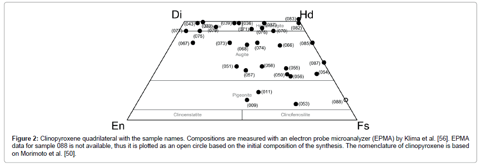
Figure 2: Clinopyroxene quadrilateral with the sample names. Compositions are measured with an electron probe microanalyzer (EPMA) by Klima et al. [56]. EPMA data for sample 088 is not available, thus it is plotted as an open circle based on the initial composition of the synthesis. The nomenclature of clinopyroxene is based on Morimoto et al. [50].
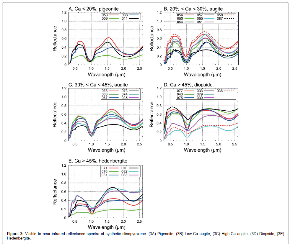
Figure 3: Visible to near infrared reflectance spectra of synthetic clinopyroxene. (3A) Pigeonite, (3B) Low-Ca augite, (3C) High-Ca augite, (3D) Diopside, (3E) Hedenbergite.
Deconvolution with the exchange Monte Carlo method
Deconvolution results of pyroxene spectra are shown in Figure 4. The best optimized parameters for 1, 1.2, and 2 μm bands are summarized in Table 1. Errors estimated from 2σ based on ten runs using different series of random numbers are also shown. Most of the spectra are best fitted by 4 to 6 Gaussians with appropriate continuum. For example, sample 053 is fitted with 4 Gaussians with their centers locating at 0.091, 0.965, 1.258, and 2.180 μm and a nearly constant continuum. For pigeonite and augite, our results show that the spectra are mainly fitted with 3 Gaussians with their centers locating at about 1, 1.2, and 2 μm, and with one Gaussian in the wavelength region ranging from ultraviolet to visible and with a continuum being nearly constant or gradually decreasing toward shorter wavelengths (Figures 5a-5d). Each Gaussian function could be physically interpreted to represent spin-allowed crystal field transitions with 1 μm for Fe2+ in the M1 and M2 sites, 1.2 μm for Fe2+ in the M1 site and 2 μm for Fe2+ in the M2 site (Figures 6a-6d). A Gaussian in the wavelength region ranging from ultraviolet to visible could represent oxygen-metal charge transfers which are centered within the ultraviolet region [34] (Figure 7). Although additional small bands centered near 0.7 μm may be necessary to improve the fitting such as shown in sample 054, we find that the additional band does not significantly affect the band center for 1, 1.2, and 2 μm absorptions. Our deconvolution results for pigeonite and augite are consistent with those by Klima et al. [56].
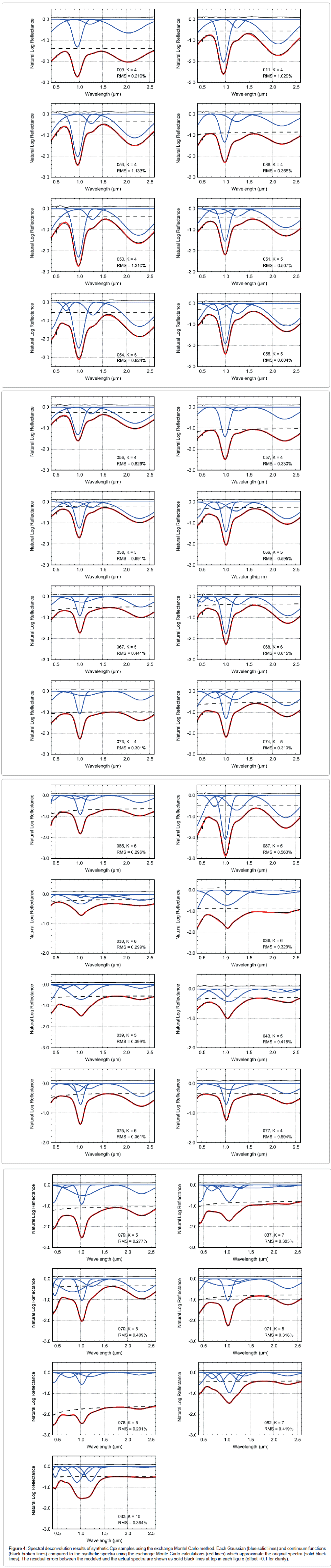
Figure 4: Spectral deconvolution results of synthetic Cpx samples using the exchange Montel Carlo method. Each Gaussian (blue solid lines) and continuum functions (black broken lines) compared to the synthetic spectra using the exchange Monte Carlo calculations (red lines) which approximate the original spectra (solid black lines). The residual errors between the modeled and the actual spectra are shown as solid black lines at top in each figure (offset +0.1 for clarity).
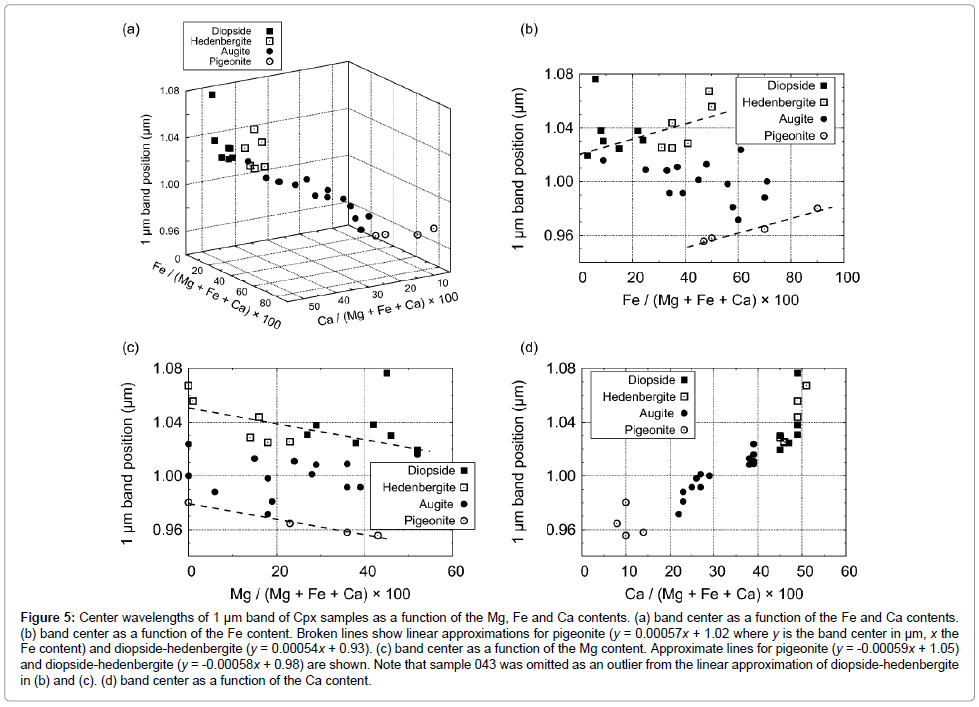
Figure 5: Center wavelengths of 1 μm band of Cpx samples as a function of the Mg, Fe and Ca contents. (a) band center as a function of the Fe and Ca contents. (b) band center as a function of the Fe content. Broken lines show linear approximations for pigeonite (y = 0.00057x + 1.02 where y is the band center in μm, x the Fe content) and diopside-hedenbergite (y = 0.00054x + 0.93). (c) band center as a function of the Mg content. Approximate lines for pigeonite (y = -0.00059x + 1.05) and diopside-hedenbergite (y = -0.00058x + 0.98) are shown. Note that sample 043 was omitted as an outlier from the linear approximation of diopside-hedenbergite in (b) and (c). (d) band center as a function of the Ca content.
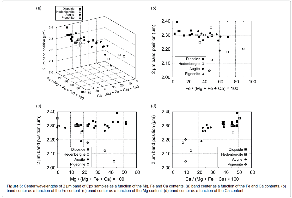
Figure 6: Center wavelengths of 2 μm band of Cpx samples as a function of the Mg, Fe and Ca contents. (a) band center as a function of the Fe and Ca contents. (b) band center as a function of the Fe content. (c) band center as a function of the Mg content. (d) band center as a function of the Ca content.
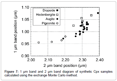
Figure 7: 1 μm band and 2 μm band diagram of synthetic Cpx samples calculated using the exchange Monte Carlo method.
Deconvolution analyses for type-A spectra including some of the diopside and hedenbergite are not as straightforward as type B, since the 1 μm bands are too narrow or too wide for a single Gaussian to fit, and some of the 1 and 2 μm bands are asymmetrical. The non-Gaussian shape of type-A spectra results in larger errors of band parameters when compared to type-B spectra (Table 1). Also, more Gaussian functions are needed to fit type-A spectra, reflecting the complex shape of the spectra. For example, samples 037 and 082 were fitted with 7 Gaussians, while sample 083 with 10 Gaussians of which 4 Gaussians are centered below 0.5 μm. Comparing our fitting results of sample 082 and 083 with those reported by Klima et al. [56], we find that the exchange Monte Carlo method yields more symmetrical configurations for Gaussians in 1 μm band. We also find that our optimal deconvolution results for samples 082 and 083 do not require the very weak absorption bands which were assigned as M2 absorptions in Klima et al. [56]. These M2 absorptions in Klima et al. [56] are significantly weak compared with the strongest M1 absorption in 1 μm band, and the M2 absorption near 1 μm was mostly covered with the M2 absorptions. For type-A spectra, it is difficult to resolve the discrepancy between the results obtained by Klima et al. [56] and this study, however, since both of the modeling results can reproduce the observed spectra almost equally well. Nevertheless, the large errors of band parameters for type-A spectra indicate that caution should be taken when performing spectral deconvolution for type-A spectra using MGM. Thus, being able to estimate errors in the fitting results based on random initial parameters is also an advantage of the exchange Monte Carlo method for assessing the statistical robustness of fitting results, which has not been performed by previous MGM analyses.
Band shift as functions of Ca, Fe, and Mg Contents
The center positions of Gaussian functions corresponding to 1, 1.2, and 2 μm absorptions are summarized in Table 1. Position shifts of 1 μm band as functions of Ca, Fe, and Mg components (solid solution) are shown in Figure 5, while position shifts of 2 μm band are shown in Figure 6. Our results are found to be consistent with those of Klima et al. [56], suggesting that the exchange Monte Carlo method developed in this study is able to extract results similar to those obtained by conventional MGM analysis.
The band centers of 1 μm absorption have a linear dependence on Wo (Ca/(Mg+Fe+Ca) molar%) contents, moving to longer wavelengths with increasing Wo. For diopside and hedenbergite with Wo ≈ 50, the band centers of 1 μm absorption largely scatter within the range of 1.03-1.08 μm. Pigeonite also shows a large variance as a function of Wo component, however, the band centers of 1 μm absorptions have a linear dependence on En (Mg/(Mg+Fe+Ca) molar%) or Fs (Fe/(Mg+Fe+Ca) molar%) components. The band centers of 1 μm absorption of augite scatter widely as a function of Fs content, and distinct dependence on Fs content were not observed. For diopside and hedenbergite samples, with the exception of sample 043, the band centers of 1 μm absorptions seem to have a linear dependence on Fs content, moving to longer wavelengths with increasing Fs content. En content seems to have no obvious influence on the band center of 1 μm absorption, except for pigeonite. We find that pigeonite, augite and diopside-hedenbergite can be separated with the use of 1 μm band position as a function of Fs or En content, as shown in Figure 5.
The band centers of 2 μm absorption seem to follow an approximation line on the space of Fs and Wo contents (Figure 6a). The band centers of 2 μm absorption for pigeonite and augite move to longer wavelengths with an increase of Wo content. The average center wavelengths of 2 μm absorptions for diopside and hedenbergite remain almost constant at around 2.3 μm, but they scatter significantly around the average value, reflecting the asymmetry shape of 2 μm absorptions for some of the type-A spectra. The band centers of 2 μm absorptions of pigeonite move longer wavelengths with increasing Fs content. Overall, the band center of 2 μm absorption is separated between low- Ca clinopyroxene (pigeonite) and high-Ca pyroxene (augite, diopside, and hedenbergite) with a gap from 2.20-2.25 μm. Klima et al. [56] interpreted the gap to be a transition zone of mineral structure between P21/c and C2/c. Our results generally agree with their interpretation with one exception, i.e., sample 056 is assumed to be pigeonite in Klima et al. [56].
The diagram between 1 μm and 2 μm band positions is shown in Figure 7. Generally low-Ca pyroxene locates in a shorter wavelength region, while high-Ca pyroxene locates in a longer wavelength region [19,41,52,56]. Our results are consistent with previous studies based on MGM analysis [41,56].
In order to avoid the local minimum problem, a Bayesian spectral deconvolution method with the exchange Monte Carlo algorithm has been applied to visible to near infrared reflectance spectra of synthetic Cpx with wide ranging Mg, Fe, and Ca contents. The results obtained in this study generally agree well with conventional MGM analyses. Here, we discuss some potential interpretations for the deconvolution results, as well as the discrepancies with previous results obtained by MGM analyses.
Fitting type-A spectra
Type-A spectra generally appear in high-Ca pyroxene such as diopside and hedenbergite, although previous studies suggest that there is no simple relationship between chemical composition of natural pyroxenes and type-A spectra [20,52,53]. The spectral data of samples 076, 037, 083, and 036 are categorized in type-A, which lack distinctive 2 μm bands. Since the absorption near 2 μm is mainly caused by spinallowed crystal field transition of Fe2+ in the M2 site, the absence of 2 μm band from type-A spectra is interpreted as a result of the replacement of Fe2+ in M2 site by other cations such as Ca2+ and Fe3+ [52,67]. On the other hand, spin-allowed crystal field transition due to the M1 site, with the absorption center locating near 1 and 1.2 μm, appear strong, and the two bands are combined to yield single broad band around 1 μm. It is difficult to fit type-A spectra with manually provided initial parameters (e.g., center, strength of Gaussian) using a conventional MGM algorithm, since the final solutions directly depend on the initial parameters, especially for the broad 1 μm band due to its non-Gaussian shape [56]. Although it is still difficult for the exchange Monte Carlo method to delineate the optimal number of Gaussians, we find that the center wavelengths of Gaussian functions for the broad 1 μm band do not move significantly with varying K. For example, the broad 1 μm band of sample 083 was fitted with two major Gaussian functions which could correspond to crystal field absorptions due to the M1 site whose center wavelengths of absorptions locate near 1 and 1.2 μm. Although the estimated errors are large, the overall result is consistent with previous deconvolution analyses of type-A spectra [53,56], suggesting that even with manually provided initial parameters, previous analyses obtained statistically optimal results. Since manually fitting type-A spectra is more difficult than type-B spectra, the exchange Monte Carlo method can be a useful tool for future deconvolution analysis for type-A spectra, of which are likely to appear in high-Ca pyroxene [52,53]. In addition, natural Cpx incorporate many minor compositions such as Al, Ti, Mn and Cr [49,50]. Such minor elements in natural Cpx yield more complex spectra than synthetic Cpx, thus the scheme presented in this paper can be useful to deconvolve such spectra.
1 μm band position vs. Ca-Fe-Mg content
Figure 5a indicates that the Cpx seem to follow a linear relationship among the 1 μm band position, with Fs and Wo contents. As shown as broken lines in Figures 5b and 5d, linear relationships are observed for pigeonite and diopside-hedenbergite with their Fs or En content. It should be noted that for diopside-hedenbergite, linear approximation was performed for all of the samples except sample 043. Sample 043 was omitted as an outlier because the spectrum shows higher reflectance and weaker absorptions compared with other samples, generally suggestive of the effect of glass [16,56,68]. Although it has been well documented for low-Ca pyroxene that the linear dependence of 1 μm band centers on Fs or En content [19,41,52,54,56], the relationship between the 1 μm band center and Fs or En content for high-Ca pyroxene has been poorly constrained by MGM analyses. Clénet et al. [41] analyzed only two high-Ca natural pyroxene samples in the diopside-hedenbergite region, thus no clear relationship has been derived. Although Klima et al. [56] analyzed 13 high-Ca pyroxene samples in the diopsidehedenbergite region; they observed no clear relationship between the 1 μm band center and Fs or En content. Our analyses show that the 1 μm band center of high-Ca pyroxene (i.e., diopside and hedenbergite) depends on Fs or En content with the band center moving longer wavelengths with increasing Fs content. This tendency is similar to the relationship between the 1 μm band center and the Fe/Mg ratio of Cafree orthopyroxene [64]. For Ca-saturated synthetic Cpx in which most of the M2 site is dominated by Ca2+, varying Fe/Mg ratio would affect only Fe/Mg in the M1 site because the M2 site is dominated with larger Ca2+ cations. Thus, the change of Fe/Mg would appear only in the 1 μm band center caused by a crystal field transition in the M1 site, but not in the 2 μm band center caused by the absorption due to the M2 site. We note, however, that large errors are included in the modeling results for type-A spectra (Table 1), thus additional data is necessary to confirm our interpretation.
Band center in three-dimensional spaces
As mentioned above, both the 1 μm and 2 μm bands seem to plot on approximate lines in the three-dimensional (3D) space of Fs-Wo content (Figures 5a and 6a). Low-Ca pyroxene samples (pigeonite) used in this study locates in the high-Fe and low-Ca regions with both the band centers being at shorter wavelengths. On the other hand, high-Ca pyroxene samples (diopside and hedenbergite) used in this study locates in the low-Fe and high-Ca regions with both the band centers being at longer wavelengths. Augite with intermediate-Wo contents distribute a in a linear trend between low-Ca and high-Ca pyroxene. Each mineral group displays three distinct clusters on these 3D spaces. The linear trend seen in both 1 μm and 2 μm bands could be understood from a crystallographic point of view. Whereas high-Fe and low-Ca Cpx samples contain more Fe2+ cations in both the M1 and M2 sites, leading to a decrease of the bond lengths due to the smaller size of Fe2+, which results in an increase in the crystal field splitting [34,69,70], low-Fe and high-Ca Cpx samples have larger Ca2+ cations, which dominate the M1 and M2 sites, leading to an increase in the bond lengths and a decrease in the crystal field splitting.
Application to future remote reflectance spectroscopy
Despite requiring meticulous parameter adjustment and prior information of mineralogy, MGMs using gradient descent method have been applied to reflectance spectra not only of laboratory data but also remote sensing data of the Moon [71], Mars [4,6,72-75], and some asteroids [76,77]. By applying the exchange Monte Carlo method to spectra of synthetic Cpx samples, we have shown that it is able to yield results consistent with both conventional gradient descent methods and crystal field theory. This means that the exchange Monte Carlo method could be applicable to at least some of the previous remote sensing data which have been analyzed using conventional MGM methods. Because the application of MGM analyses has been limited due to meticulous parameter adjustment, the exchange Monte Carlo method may have a potential to expand the applicability of MGM to a variety of space/ground-based observations, especially when we cannot obtain prior information of the target body beforehand. Remote sensing data of terrestrial reflectance spectroscopy have been validated with various reference spectra observed by in situ sample analyses, increasing the confidence of interpretation of remote sensing data [12,17,78,79]. However, such an analysis is not always available due to various geological contexts. The situation is more serious for space/ ground-based observations of small bodies in the solar system, because reflectance spectra are the only available compositional information for most of the small bodies such as Phobos, Deimos [80,81] and asteroid 1999 JU3 which is the target of Japanese space mission Hayabusa 2 [82]. In fact, asteroids are clustered based solely on reflectance spectra, although their detailed mineral compositions are poorly constrained [83]. Considering the large number of small bodies in the solar system, it is unlikely to send probes to each small body to conduct in situ sample analysis or sample return. Given the limited data and resource, interpreting reflectance spectra without assuming a priori information is essential not only for planetary science but also for mission planning. The exchange Monte Carlo method could be significantly useful under such circumstances, where meaningful compositional information other than reflectance spectra is not available.
We applied a Bayesian spectral deconvolution method with the exchange Monte Carlo algorithm to visible/near infrared reflectance spectra of synthetic clinopyroxene of diverse compositional variation, in order to avoid the local minimum problem and to remove the arbitrariness originated from initial parameters, inherent in the previous Modified Gaussian model. Our results indicate that the exchange Montel Carlo method is able to yield the consistent results obtained by conventional Modified Gaussian model. Since our model does not rely on a preliminary knowledge of the reflectance spectrum of mineral, the results suggest that previous spectrum analyses have obtained statistically optimal results. The successful application of our model to reflectance spectra of minerals indicates that this model could be applied to an automatic deconvolution analysis for a large spectral database, especially useful for space missions when preliminary knowledge of mineralogy is not available. Given the recent and future advancement of space missions, the exchange Monte Carlo method could be a useful tool for analyzing a wide range of minerals and remote sensing data of rocky bodies in the solar system.
This research utilizes spectra acquired with the NASA RELAB facility at Brown University. This work is supported in part by JSPS grant-in-aid 25120006 and TeNQ/Tokyo-dome.