Advances in Automobile Engineering
Open Access
ISSN: 2167-7670
ISSN: 2167-7670
Research Article - (2016) Volume 5, Issue 2
Center pivot irrigation system has the potentiality for economically net –return of various crop patterns, although it’s higher fixed costs inputs. Therefore, water management under the specified center pivot irrigation system can play a crucial role in maximizing water unit productivity and enhancing physical-agricultural resources sustainability. Hereby, the aim of this research was to evaluate the optional of a general reflectance model based solely on soil moisture distribution pattern as a key for on-farm irrigation management under center pivot irrigation system. Data revealed that the relative reflectance was strongly correlated with soil moisture contents. However, the best correlation was found act high soil moisture level between the reflectance values of 700 nm (Red-NIR) wave length and the volumetric water content (R² = 0.9). Moreover, the observed data could help to quality the strong in influence of soil moisture on spectral reflectance and absorption features and should aid in the development operational and management algorithms of on-farm irrigation systems.
<Keywords: Center pivot irrigation; Relative reflectance; Irrigation system; Soil moisture
Understanding of soil hydraulic properties and characteristics are crucial for the solution of equations describing the water management under unsaturated soil conditions of the irrigated agriculture in arid regions. However, the accurate estimated of water flux and therefore water availability is of importance environmental issues. Water retention curves describe the relationship between the pressure head and the volumetric water content. Particle size distribution data have been widely used as a basis for estimating soil hydraulic properties and consequently irrigation water scheduling. Hydraulic conductivity of unsaturated soil is one of the most important soil properties controlling infiltration and surface runoff, as well as leaching of the applied agro-chemicals. Hydraulic conductivity depends strongly on soil texture, structure and therefore can vary widely space. Several methods have been developed to investigated and estimate, as well as simulate the soil hydraulic properties from more easily measured soil properties. Some of these methods were described by [1]. Soil moisture is an important factor across a range of environmental processes, including plant growth, soil biogeochemistry, land – atmosphere heat and water exchange [2-4]. Therefore timely and accurate measurements of soil moisture are highly described for on farm irrigation water management. However monitoring of soil moisture distribution uniformity under center pivot irrigation system is highly required for understanding and modeling irrigation systems and maximizing on farm irrigation water unit net return. The uniformity of water application under a center pivot is determined by setting out cans or rain gauges along the length of pivot, bringing the irrigation system up to proper operating pressure, and letting the system pass over them (Record the distance from the center of the pivot and the amount of water collected for each can or gauge. From this information, a coefficient of uniformity can be calculated. The coefficient of uniformity is usually expressed as a percentage [5].
Remote sensing approaches have primarily focused on microwave wavelength, where moisture exerts strong control over soil dielectric properties and where measurements are not impeded by clouds or darkness [6,7]. On the other hand, moisture influences the reflection of shortwave radiation from soil surfaces in the VNIR (400-1100 nm) and SWIR (1100-2500 nm) region of the spectrum (Skidmore et al., 1975). However, quantification of moisture using these wavelengths remains difficult because of significant variability from other soil chemical and physical properties, such as organic matter and mineralogy, as well as vegetation cover [8]. Khairallah et al. [9] investigated the relationship between soil moisture content and soil surface reflectance and indicated that it is feasible to estimate surface (0 to 7.6 cm) soil moisture from visible to near infrared reflectance. However, the main objective of this study was to monitor temporal and spatial changes, in the field water application uniformities along radial and circular lines from center-pivot systems using spray nozzles using soil reflectance as a soil proceeded from wet to dry states and to determine the dependence of these changes on wavelength. Romaguera et al. [10] stated that the volume of water consumed for its production is defined as crop Water Footprint (WF). However, the volume of irrigation applied calculated by mass water balance, and green and blue WF obtained from the green and blue evapotranspiration components. In addition, the combination of data brings several limitations with respect to discrepancies in spatial and temporal resolution and data availability could represent an innovative approach to irrigation mapping. With this point of view, Gutierrez et al. [11] used spectral reflectance indices to estimate the water status of plants in a rapid, non-destructive manner. Water spectral indices as normalized water index NWI were measured on wheat under a range of water-deficit conditions in field-based yield trials to establish their relationship with water relations parameters, as well as, available volumetric soil water (AVSW) to indicate soil water extraction pattern. Therefore, Droogers et al. [12] stated that the irrigation application amounts can be estimated reasonably accurately, providing data are available at an interval of 15 days or shorter and the accuracy of the signal is equal or higher 90%.
Therefore, the aim of this study was to attempt to use soil-spectral reflectance technique under arid conditions for monitoring and managing of irrigation water under arid conditions of Egypt.
Experimental layouts and site descriptions
Field experiments were carried out in the Experimental Farm of Faculty of Agriculture, Ain Shams University, El-Kanater city, Kalubia Governorate, under a single-span center-pivot irrigation system. The studied area is located between longitude 30º 12’ 53”, 30º 12’ 53”, 30º 12’ 50”, 30º 12’ 51” - E and latitude 31º 08’ 01”, 31º 07’ 57”, 31º 08’ 58”, 31º 08’ 01” - N. However, soil-physical and Hydro-physical characteristics of the investigated site had been illustrated in Table 1.
| Sample depth (cm) |
H.C (cm/h) |
Particle size distribution (%) | Ɵ % | BD (g/cm3) |
|||||
|---|---|---|---|---|---|---|---|---|---|
| Coarse sand | Fine sand | Clay | Texture class | F.C | P.W.P | A.W | |||
| 0-5 | 0.9 | 25.8 | 41.5 | 30.8 | SCL | 31.46 | 15.10 | 16.36 | 1.25 |
| 5-10 | 1.0 | 25.5 | 40.2 | 33.3 | SCL | 31.21 | 15.42 | 15.97 | 1.28 |
Table 1: Some physical properties of the soil at the experimental site.
Calibration of reflectance spectrometer
Due to the variations in the manufacture of the electrical components, lamps, and light sensor, of the readings of this instrument must correct. To correct for these differences between instruments and to move the measurement closer to what happens to the light, measurement of light reflectance is given as the percentage or proportion of light (for each wavelength or color) that reflects from the soil. The display number measurements indicate how much light (of each color) has reflected from the soil, but how much light hit the soil to start with. One way to measure how much light hits the soil and how much is reflected, is to take reflectance measurements of a standard material. Good standards for this experiment are heavy white paper or white poster board, which reflect almost all of the light that hits them, about 85%.
With the “Standard” data, we can now calculate the proportion (or percentage) of light reflected by the soil. For each color, simply divide the display voltage number for the soil by the display voltage number for the white paper. This value is called the reflectance.
Reflectance = (Display number for sample) / (Display number for white paper).
To convert this reflectance proportion to a percentage, simply multiply by 100. Displayed numbers for white paper using different wave lengths are 646, 800, 790, and 836 for 470, 560, 600 and 700 Aº respectively. However, soil water uniformity distribution under center pivot irrigation system had been measured in order to evaluate the efficiency of the portable reflectance spectrometer in detecting water content of the surface layer of the soil within different times of soil depletion up to 96 hrs after shutdown of the irrigation events comparing with the reading of the standard calibration method. However, the investigated time had been selected according to the scheduling time of sprinkler irrigation systems, under arid conditions of Egypt. The observed calibration data and observed correlation equations had been represented in Figure 1 and Table 2.

Figure 1: Soil reflectance in different wavelengths as affected by the time.
| Time of investigation | R2 | Equation |
|---|---|---|
| 24 hrs | 0.0371 0.2795 0.474 0.6597 |
% reflectance at 470nm = 13.426Ɵ + 15.663 % reflectance at 560nm =41.131Ɵ + 1.9798 % reflectance at 600nm= 55.736Ɵ - 1.7173 % reflectance at 700nm = 45.88Ɵ + 0.9741 |
| 48 hrs | 0.1316 0.0039 0.3582 0.241 |
% reflectance at 470nm= 14.73Ɵ + 11.058 % reflectance at 560nm = 3.3619Ɵ + 15.561 % reflectance at 600nm= 25.153Ɵ + 7.2439 % reflectance at 700nm= 17.575 Ɵ + 10.496 |
| 72 hrs | 0.014 0.0297 0.0099 0.1078 |
% reflectance at 470 nm = -7.7771 Ɵ + 18.96 % reflectance at 560nm= 6.827Ɵ + 12.675 % reflectance at600nm = 4.1823 Ɵ + 15.389 % Reflectance at 700nm= 9.7053Ɵ + 12.932 |
| 96 hrs | 0.0383 0.0163 0.009 0.1303 |
% Reflectance at 470nm= -12.103Ɵ + 20.544 % Reflectance at 560nm = 6.3585Ɵ+ 12.768 % Reflectance at 600nm= 3.9487Ɵ + 15.052 % Reflectance at 700nm = 9.1656Ɵ + 12.776 |
Table 2: The correlation coefficients (R2) and the linear equations for the relationship between the volumetric watercontent and the percent of soil-spectral reflectance.
Multiple linear regression analysis using stepwise selection method
Two statistical analyses were employed in this study, the multiple linear regression (MLR) method and Stepwise selection method.
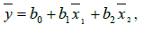
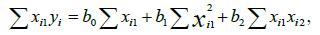
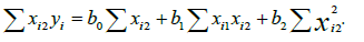
Multiple linear regressions (MLR): A stepwise multiple linear regression analysis used predicts the Coefficient of uniformity CU and crop evapotranspiration ETc values by vegetation indices VI’s and water indices WI’s multiple linear regressions involves the fitting of a response to more than one predictor variable. For example, an experimenter may be interested in modeling (y) as a function of some properties, including (x1), (x2), and (x3). A benefit of the modeling of a response as a function of two or more predictor variables is flexibility for the analyst. A wider variety of response variables can be satisfactorily modeled with multiple regression models than can be with single variable models. In a single variable analysis, one is confined to using functions of only one predictor. In multiple regression analyses, different individual and joint functional form for each of the predictors permitted. Direct comparisons of alternatives of predictors also can be made. Multiple linear regression models can be defined as follows Equation. 27. The sum of the squared residuals SSE is given by Equation. 28, and the normal equations for a model having p = 2 predictor variables showed in equation 29,30 and 31.
 (27)
(27)
ei is the error of the model.
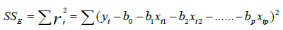 (28)
(28)
 (29)
(29)
 (30)
(30)
 (31)
(31)
Stepwise selection method: Stepwise selection methods sequentially add or delete predictor variables to the prediction equation, generally one at a time. These methods involve fewer model fits than all possible subsets, since each step in the procedure leads directly to the next one. There are three popular subset selection methods using stepwise selection are forward selection, backward elimination, and stepwise iteration. The forward selection (FS) procedure for variable selection begins with no predictor variables in the model. Variables are added one at a time until a satisfactory fit is achieved or until all predictors have been added. At each step of the selection procedure only one model is fitted: the reduced model containing all predictors not yet deleted. The backward elimination (BE) procedure for variable selection begins with all the predictor variables in the model. Variables are deleted one at a time until an unsatisfactory fit is encountered. At each step of the selection procedure only one model is fitted, the reduced model containing all predictors not yet deleted. The stepwise iteration (SI) procedure adds predictor variables one at a time like a forward selection procedure, but at each stage of the procedure, the deletion of variables is permitted. It combines features of both forward selection and backward elimination More computational effort is involved with stepwise iteration than with either forward selection or backward elimination The tradeoff for the additional computational effort is the ability to delete non-significant predictors as variables are added and the ability to add new predictors following deletion [13].
Figure 2 represents the volumetric water content distribution under the center pivot irrigation system as affected by either time after soilmoisture stability time 24 h, 48, 72 and 96 hrs or the distance from the center pivot. Soil- moister contents in the middle distance point, 50 m, were highest compared to the nearest and farthest points; 0 and 100 m, from the center pivot tower. However, all wavelengths of reflectance increased with time progress. The familiar darkening of soil upon wetting is because of a change in the real part of the refractive index (n) of the immersion medium from air (n = 1) to water (n = 1.33) [14,15]. This decrease of the contrast between soil particles (n ~ 1.5) and their surrounding medium, resulting in an increase in the average degree of forward scattering and, thus, an increased probability of absorption before reemerging from the medium.

Figure 2: Relationship between soil volumetric water content (O) and the % reflectance in different wavelengths under the center pivot irrigation system.
The effect of soil moisture on reflectance was summarized for each sample points by determining the best-fit coefficients of linear relationship relating moisture and reflectance. However, the relationship between the soil moisture contents (Ɵ) and the light of reflectance at different wavelengths: 470 to 700 nm, and different time series. The data indicated that the reflectance values in the four studied wavelengths were linearly coordinated with the soil moister content after one hour. This relationship gradually disappeared with time progress till we reached 96 hr. Starting from 48 hrs, there is no correlation between reflectance values and the soil moisture content.
On the other hand, after 24h, the values of R2 decreased with decreasing the wavelength from 700 nm to 470 nm. The highest R2 values (0.6) were found between % reflectance at 700 nm and the soil moister content. This high to moderate correlation inversed to a very weak correlation which reflected on the R2 values under the other three times, 48, 72 and 96 hours. These results revealed that with decreasing the soil moister content the reflectance becomes independent from the moister and affected by other soil components. These results in agreement with those of Hillel [16] who mentioned that in visible wavelengths, the sole effect of water is in changing the relative refractivity at the soil particle surfaces.
Data analysis of the observed results
Results of the statistical analysis using the stepwise multiple linear regression to predict Volumetric Water Content with respect of hours using spectral response is demonstrated in (Figures 3 and 4) and (Tables 3 and 4). However, the statistical analyses show that high positive correlation between Volumetric Water Content with respect of hours and spectral response (0.82). Moreover correlation between Volumetric Water Content with respect of hours and spectral response at 0 mater data is respond as outlier and cause a lack of fit of the second polynomial degree equation that required to be neglected for running the equation to predict Volumetric Water Content Ɵ using spectral response [17].

Figure 3: Bivariate fit of soil-spectral reflectance and soil moisture volume based on hours of investigations.

Figure 4: Trends of soil-spectral reflectance and soil moisture volume based on hours of investigations.
| Variable | Mean | StdDev | Correlation | Signif. Prob | Number |
|---|---|---|---|---|---|
| Hours | 60 | 26.8488 | -0.82239 | <0.0001* | 840 |
| ref, vol | 18.37831 | 1.979691 |
Table 3: Correlation analysis of the relationship between measured soil moisture content and soil-spectral reflectance based on hour of investigation.
| Source | DF | Sum of Squares | Mean Square | F Ratio |
|---|---|---|---|---|
| Model | 2 | 2738.3898 | 1369.19 | 2084.421 |
| Error | 837 | 549.8007 | 0.66 | Prob> F |
| C. Total | 839 | 3288.1905 | 0.0000* |
Table 4: Analysis of the variance between measured soil moisture content and soil-spectral reflectance based on hour of investigation.
The correlation between predicted Volumetric Water Content with respect of hours and spectral response using polynomial second degree equation was quite acceptable with R2 of 0.83 (Table 5).
| Term | Estimate | Std Error | t Ratio | Prob>|t| |
|---|---|---|---|---|
| Intercept | 21.038351 | 0.076901 | 273.58 | 0.0000* |
| Hours | -0.060639 | 0.001042 | -58.19 | <.0001* |
| (hours-60)^2 | 0.0013587 | 4.855e-5 | 27.99 | <.0001* |
Table 5: Parameter estimates.
Ref, vol = 21.038351 - 0.0606388*hours + 0.0013587*(hours-60)^2
Summary of Fit
R Square: 0.832795
R Square Adj: 0.832396
Root Mean Square Error: 0.810476
Mean of Response: 18.37831
Observations (or Sum Wgts): 840