Advances in Pediatric Research
Open Access
ISSN: 2385-4529
ISSN: 2385-4529
Research Article - (2025)Volume 12, Issue 4
Amid growing economic uncertainty, household economic resilience has become a critical issue, especially in developing countries. At the same time, child stunting and cognitive impairment remain pressing developmental challenges, disproportionately affecting households with lower socioeconomic status. This study aims to construct a comprehensive and valid index for measuring household economic resilience by employing multidimensional household characteristics. Using data from the 2014 Indonesian Family Life Survey (IFLS), we develop a latent variable representing household economic resilience through factor analysis, incorporating indicators of economic welfare, living conditions, social protection and financial literacy, each constructed from multiple constituent variables. Additionally, we explore the impact of household resilience on child growth, employing rainfall as an Instrumental Variable (IV). The findings reveal a significant reduction in the likelihood of stunting with an increase in household resilience. However, while positive, the effects on HAZ, WAZ and WHZ were not statistically significant. Notably, we observed an improvement in children's total cognitive z-score and math cognitive z-score, though past exposure to economic shocks did not produce significant results. The resilience index offers valuable insights for policymakers, helping to better target vulnerable populations and direct social protection programs and resources to those most in need.
Household economic resilience; Welfare; Well-being; Poverty; Child growth
The shifting temporal dynamics driven by climate change, natural disasters and concurrent economic disruptions have intensified the focus on household resilience, particularly in the context of heightened vulnerability. The need to address this challenge has given rise to various initiatives to establish robust metrics of economic resilience as a basic foundation for policy formulation. The application of this analytical framework has been crucial in assessing households’ capacity to withstand and adapt to various shocks, including economic disruptions. Accurate measurement of resilience stands to assist policymakers in gauging the efficacy of governmental programs, as well as in identifying the precision of their targeting strategies. Moreover, it facilitates the design of government initiatives that prioritize the alleviation of economic shocks for socioeconomically marginalized segments, particularly within developing nations [1].
A strand of studies has analyzed the concept of resilience from various disciplinary perspectives, such as economic, natural disaster, social, health and institutional. Previous research on economic resilience has predominantly focused on the macro level. While some studies have sought to assess resilience at the household level, these typically emphasize natural disaster shocks. For instance, Feeny explored household-level economic resilience by examining responses to rising food and fuel prices. However, such measures often reflect resilience as a post-shock outcome. This study aims to address these gaps by developing a household-level measure of economic resilience that incorporates factors predictive of household preparedness in the face of potential shocks.
Focusing on the Indonesian context, we construct an economic resilience index. As a developing nation, Indonesia is home to a significant population of individuals living in poverty, with 26.2 million people classified as impoverished in 2022. Households in this demographic are particularly susceptible to health-related vulnerabilities that affect multiple facets of their livelihoods. Their exposure to adverse shocks such as income declines, rising prices of essential goods and natural disasters is further exacerbated by limited resources. These risks often remain unmitigated due to resource shortages. Even for extremely poor households, resource constraints can push them into a prolonged cycle of poverty [2].
In Indonesia, the agricultural sector still dominates. What is unique about farming households is their dual function as producers and consumers. However, the dominance of net consumer farmers in Indonesia makes them vulnerable to shocks. This is supported by Warr and Yusuf who found that rural households are more vulnerable to falling into poverty as a result of food price shocks. The sector’s income is also strongly influenced by weather. Despite the significant presence of the informal sector and Micro, Small and Medium Enterprises (MSMEs) in Indonesia’s labor force, a majority of MSMEs remain informal, contributing to households’ vulnerability to shocks.
Several efforts have been made to measure resilience indices in Indonesia. However, district-level analyses from these studies are not directly applicable to households for several reasons. The large population size reflects a wide diversity of characteristics and inequality both in income and infrastructure remains a significant issue, with its effects disproportionately impacting specific groups. These nuances are often overlooked in macrolevel assessments, underscoring the need for more targeted resilience measurements at the household level.
This study measures household resilience in Indonesia using four dimensions, namely household economic welfare, living conditions, social protection net and financial inclusion. Each dimension is a latent variable that is measured based on indicator variables. The welfare dimension is assessed through various household characteristics, including years of education, the proportion of breadwinners, household expenditure, asset ownership and food security levels. The household living conditions include the availability of basic needs such as water source, toilet, television and floor type. The social protection net includes social assistance received by the household. Meanwhile, financial behavior consists of household knowledge of financial facilities and ownership of savings and/or stocks. The inclusion of this dimension is informed by a series of studies in developing countries that demonstrate the significant impact of financial literacy on welfare and poverty reduction. While the resulting resilience index can be directly utilized as a policy basis, we extended the analysis to examine the influence of household resilience on child growth. This specific variable was selected due to its potential to anticipate enduring effects on household socio-economic status, a critical factor when exploring developmental contexts within emerging economies [3].
This research contributes to policy in several ways. By defining economic resilience as households’ ability to overcome shocks, the generated resilience index in Indonesia acts as a government tool to pinpoint areas for enhancing household economic resilience pre, during and post-shocks, minimizing potential risks. Additionally, the economic resilience framework, coupled with social protection indicators, aids in precisely evaluating program targeting. In instances where low-resilience households lack program assistance, it necessitates a government review and realignment of interventions to address these vulnerable areas. Secondly, this study uniquely gauges economic resilience at the household level, distinguishing it from previous macro-level assessments. Notably, macro-level indicators hinge on household reactions to shocks. While some studies have explored household-level measurements, they often focus on natural disaster-related shocks.
Third, to further analyze and test the obtained resilience index, we proceeded to examine its impact on child growth, gauged through cognitive capacity and stunting measurements. Although external risk factors experienced by children have a substantial and prolonged impact on the future, very few studies have investigated the relationship of household resilience to child growth. This aspect of development economics was chosen because it has a sustained and intergenerational impact on the socioeconomic status of households, which is a concern in policy-making in developing countries. Existing policies that focus on this aspect tend to emphasize nutrition programs themselves and access to health facilities as demand-side policies. Examining the impact of economic resilience on child growth stands to make a substantive contribution to the formulation of policies addressing poverty and developmental concerns [4].
Construction of economic resilience index
Previous studies have measured economic resilience to inform the adoption of the estimation model. Given the abstract nature of resilience, some of these studies have been criticized and have been refined in subsequent studies. Cisse and Barrett, for instance, constructed a resilience score by examining the interaction between the probability of nonlinear poverty dynamics and poverty traps, using livestock ownership as a proxy for well-being. Their approach measured resilience by calculating the likelihood of households surpassing normative well-being thresholds under shock conditions. While this complex model is valuable for forecasting, it relies on a single resilience characteristic expressed as a probability.
An alternative method for predicting economic resilience is to utilize the latent variable framework. Economic resilience qualifies as a latent variable due to its conceptual nature, as latent variables are typically regarded as theoretical constructs that cannot be directly measured. Economic resilience, characterized as the capacity of households to withstand and adapt to shocks, defies direct quantification. This parallels the concept of quality of life, which, though intangible, is inferred through a suite of indicators encompassing socioeconomic dimensions, health and more. To generate latent variables, several statistical techniques can be utilized, namely factor analysis and Principal Component Analysis (PCA) [5].
Factor analysis and Principal Component Analysis (PCA) are two statistical techniques designed to reduce dimensionality. Both techniques leverage several indicator variables to generate a latent variable, which, in this context, represents economic resilience. Unlike Cisse and Barrett, who define resilience as a shift in normative well-being or poverty levels, factor analysis and PCA enable the prediction of resilience based on a broader set of relevant factors. Although their objectives and procedures are similar, the techniques differ fundamentally. PCA generates new, uncorrelated variables from the original indicators, while factor analysis identifies latent variables or factors, inherent in the correlated indicator variables, which are then extracted as new variables.
Table 1 shows a more detailed comparison between the three methods. Given that PCA generates latent variables byemphasizing the most prominent variation in the dataset, it follows that the selection of indicator variables need not conform to a predetermined pattern or rationale. PCA “forces” all components to explain the correlation structure of the indicators. Meanwhile, factor analysis produces latent variables that are more “realistic” because they are “drawn” from the relationships between indicator variables. This study utilizes a two-stage factor analysis to generate an economic resilience index. In the first stage, we calculated the latent variable value of each sub-indicator. Then, factor analysis in the second stage will produce an economic resilience index.
|
|
C and B (Cisse and Barrett) resilience measurement |
Principal Component Analysis (PCA) |
Factor Analysis (FA) |
|
Objective |
C and B treats resilience as a dependent variable. The C and B method compares each household’s resilience score, with the minimum acceptable likelihood of achieving some normative welfare standard, such as the poverty line |
PCA, a dimension reduction technique, minimizes dimensionality while preserving information in the original data. It transforms variables into orthogonal components that capture the most variance |
Like PCA, FA is a dimensionality reduction technique. It uncovers latent variables (factors) underlying some indicator variables, aiding in identifying data patterns. FA serves both explanatory purposes by revealing data structure and confirmatory purposes by validating theoretical relationships between variables |
|
Mechanism |
C and B utilizes OLS regressions to estimate household welfare variables’ mean and variance based on characteristics, shocks, or risk exposure. This informs the probability of a household meeting or surpassing a predefined normative standard, e.g., poverty line |
PCA generates weights (eigenvectors) for indicator variables, which are then utilized to derive latent variables explaining the overall data variation. In essence, PCA yields a summary latent variable based on its indicators |
FA does not predict a latent variable from observed variables; instead, it assumes the existence of latent variables among correlated indicators. The latent variable value is derived after running factor loadings |
|
Advantages and disadvantages |
(+) Consider nonlinear dynamics within a first-order Markov process, aligning with the empirical literature on poverty dynamics estimation |
(+) PCA assigns weights to indicators without assuming an underlying latent variable structure. (-) Sensitive to outliers and missing data |
(+) Unlike PCA, it doesn't force all components to account for the correlation structure |
|
(-) Analysis requires panel data (lags) and time series analysis |
|
(-) Too strong correlations between indicator variables can make it difficult to identify latent factors |
|
|
Data type |
The regression outcome is a probability so the data type is binary. However, other characteristics can be categorical or continuous |
Continuous data only |
Continuous data only |
|
Categorical data only (MCA/multiple correspondence analysis) |
Binary data only (Tetrachoric correlation) |
||
|
Combination of continuous and categorical data (PCAmix) |
Ordinal data only (Polychoric correlation) |
||
|
Combination of continuous and categorical data (FAMD/factorial analysis of mixed data) |
|||
|
Sources |
(Cisse and Barrett, 2018) |
(Bro and Smilde, 2014) |
(Kim and Mueller, 1978) |
Table 1: Comparison of methodologies for building economic resilience indices.
Conceptual framework: Indicators of household economic resilience
As a developing country, Indonesia often grapples with lower socio-economic conditions among its population, making them more vulnerable to unforeseen disruptions. The prevalence of rural areas compounds challenges for households in the face of shocks, stemming from uneven development in small villages. With a predominantly agricultural and informal sector, households remain vulnerable due to income fluctuations and external factors such as weather. Assessing household resilience requires examining indicators beyond mere socio-economic status, encapsulated in the broader concept of “resilience.”
The term resilience was initially analyzed by Holling who explored the resilience of natural dynamics. He defined resilience as the persistence of a perturbed entity to maintain its position within its environment. Since then, resilience has been measured across various levels, including individuals, households, villages, districts and institutions. The resilience framework is not confined to economic policy but extends to various fields where significant disruptions affect the subject’s activities. Although many resilience measurements have been made, defining resilience and putting it into a quantitative measurement is still ambiguous and challenging. This arises from the complexities involved in accurately assessing and capturing the true essence of resilience [6].
Despite resilience’s abstract nature, the inevitability of various shocks, such as natural disasters, economic downturns, civil conflicts and health crises, necessitates a tool for assessing survival capability in these situations. Resilience measurement can be the foundation of government policy to identify program targets to increase household resilience capacity. The results of this analysis can then be used to minimize the risk of shocks that may arise, especially for households with low socioeconomic status and prevent them from falling into poverty.
This research develops an Indonesian resilience index based on four dimensions. The first dimension, household economic well-being, assesses satisfaction with economic factors affecting resilience. Economic well-being correlates directly with the ability to withstand economic shock. To provide a comprehensive measure of economic resilience, the index includes household farm assets alongside traditional indicators such as expenditure and overall assets, which are particularly relevant in an agrarian context like Indonesia. Additionally, the index incorporates food security and the education level of the household head.
In assessing economic resilience, living conditions, closely tied to socioeconomic status, serve as an additional dimension. Inadequate access to basic amenities elevates the risk of economic shocks significantly. The presence of sufficient facilities also influences household preparedness for economic shocks. Social protection, alongside basic amenities, is crucial for determining households’ coping capacity. In Indonesia, social safety net policies focus on poverty reduction. Including governmental initiatives in resilience measurement facilitates assessing program efficacy, as confirmed by studies such as Abay et al. in Ethiopia and Mujuru et al. in South Africa, demonstrating increased resilience with higher household transfers [7].
Measuring economic resilience also needs to include financial literacy. Forms of loans such as microcredit that can be utilized by vulnerable households are an effort to provide equal access to financial facilities that then contribute to improving household micro-enterprises and alleviating poverty. A study in Kenya by Yao et al. was conducted to investigate the role of financial services on household economic resilience. Their findings showed a positive and significant relationship between financial access and resilience. These results were supported by Suri et al. who found that households with access to digital loans were significantly better able to survive under shocks (Figure 1).

Figure 1: Construct of economic resilience indicators.
Resilience is intricately linked to socioeconomic status, with households of lower socioeconomic status being more reliant on agriculture and government transfers. Such households are also more susceptible to falling back into poverty due to economic shocks, highlighting their vulnerability. Research studies have demonstrated the significant impact of household vulnerability on various economic development outcomes, including child growth. However, the role of resilience in mitigating these vulnerabilities remains underexplored. Specifically, there is a need to investigate the conditions under which households can be considered resilient enough to offset the risks associated with low socioeconomic status. In this study, we use child growth as an indicator to assess the vulnerabilities that households face when confronted with shocks.
Data
We utilize the data from the Indonesian Family Life Survey (IFLS), collected by the RAND Corporation. The survey has been administered in five waves: 1993/1994, 1997/1998, 2000/2001, 2007/2008 and the most recent in 2014/2015. For this study, we focus on the cross-sectional data from the 2014/2015 wave. We employed household characteristics to construct an economic resilience index and used individual characteristics to analyze child growth and cognitive development. Due to missing data, the dataset for the economic resilience index includes 8,009 households. This data was combined with individual child data, resulting in 3,598 samples of children under five years old for stunting analysis and 8,027 samples of children aged 7-14 years for cognitive ability analysis [8].
To analyze the relationship between economic resilience and various outcomes, we use rainfall as an instrumental variable. Rainfall data was sourced from Climatic Data Online (CDO) via the National Oceanic and Atmospheric Administration (NOAA) portal. The precipitation data is provided as a highresolution monthly time series with a degree of 0.5 × 0.5 grid, spanning from 1980 to 2014. For our analysis, we utilize the 2014 precipitation data and integrated it with IFLS5 data by aligning sub-districts based on their longitude and latitude.
Measurement of household economic resilience index
Figure 1 illustrates the dimensions and indicators utilized in constructing the household economic resilience index. Thus, the resilience index for household h, REh, is expressed as:

Resilience is a latent variable whose value is determined by the four indicators above. Meanwhile, the value of these indicators is also determined by their sub-indicators. This research utilizes two-stage factor analysis in determining the values of these latent variables. This method assumes that the observed variables (indicators) are linear combinations of several underlying factor variables. The emphasis on factor analysis is to explain the correlation between variables. When analyzing n variables, each correlated variable is expressed as a weighted sum of one or more latent factors (or more, as long as n<r, where r is the number of factors), with any remaining variance attributed to error. The derived latent factors reveal the underlying intercorrelations among the variables.

where h are scoring coefficients generated from factor loadings. The resilience index is then standardized using minimummaximum formation. This process results in values spanning from 0 to 1, wherein higher index values correspond to heightened levels of resilience.
We encounter 3,498 missing values of agricultural asset data due to subsampling in the interview process. However, according to information from RAND, the agriculture questionnaire was exclusively administered to farmers. With this assumption, we replaced the missing values with zero. On the other hand, missing values are observed in the variables of years of education of the household head and household assets (Table 2). To address these issues, we employ Expectation-Maximization (EM) estimation for the welfare and resilience factor analysis. The EM method estimates complete data expectations based on available data through a log-likelihood function and identifies parameters that maximize this log-likelihood expectation [9].
Estimation model
The resilience index is not associated with any measurement. In addition to predicting the resilience index, this study aims to examine the relationship between resilience and child growth. The econometric model used in the analysis is as follows:

where yihv is the outcome variable to be tracked for individual we in household h in village v, which in this context includes a number of dependent variables measuring child nutritional status, namely HAZ, WAZ, WHZ; as well as several outcome variables related to child cognitive ability, namely total raw cognitive score, math cognitive score, nonverbal cognitive score, total cognitive z-score, math cognitive z-score and nonverbal cognitive z-score. β1 is the estimated parameter. The vector Χ'1ihv includes child characteristics, Χ'2ihv includes household characteristics and Χ'3ihv represents village characteristics. There are differences in the characteristics that control between the dependents of nutritional status and child cognitive ability. Meanwhile, the notation εihv represents the error.
On the other hand, to investigate the effect on the probability of a child being stunted (HAZ<-2) and severely stunted (HAZ<-3), we leveraged the following probit model,
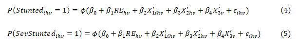
Given that the resilience index is a latent variable that is predicted from several indicators, resilience is an endogenous variable. There is a potential reverse causality, where child malnutrition can also affect household resilience. Poor nutrition in children heightens their susceptibility to illness, leading to increased health expenditures for the household, which in turn impacts its resilience. Moreover, several factors can influence both household resilience and children’s nutritional status simultaneously, such as parental knowledge, attitudes and social connections. Endogeneity issues emerge because the resilience index is inherently related to the household characteristics included in the regression model.
Endogeneity can lead to biased parameter estimates for the variables being measured. To address this issue, we employed Instrumental Variables (IV). A valid instrument should effectively predict the endogenous variables in the model while having no direct effect on the dependent variables. In this study, we use rainfall as an instrumental variable. Based on Le and Nguyen rainfall is precipitation standardized through
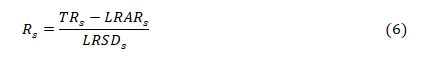
where Rs is the rainfall anomaly in subdistrict s, TRs is the rainfall level in subdistrict s. The long-term rainfall average (LRARs) and long-term rainfall standard deviation (LRSDs) are the average and standard deviation of rainfall in subdistrict s over the period from 1980 to 2014.
An instrumental variable must satisfy two key assumptions. First, the relevance assumption dictates that the instrument should significantly impact the endogenous variables. Rainfall was selected for this reason, as it has a substantial effect on the Indonesian agricultural sector, influencing farmers’ income and consequently, the vulnerability of the informal sector and MSMEs to income fluctuations related to rainfall. Therefore, variations in rainfall are pertinent in explaining household economic resilience. Second, the instrument must meet the exclusion restriction, which means it should not directly affect the dependent variables. Rainfall, while influencing agricultural production and income, does not have a direct impact on children’s health and cognition. Its effects on food availability and the incidence of diseases like diarrhea and malaria, as well as its impact on nutritional status, illustrate conditions related to household economic resilience.
Descriptive statistics
Table 2 shows the descriptive statistics of the variables to be used in constructing the household economic resilience index. Most households already have adequate drinking water sources and toilets. However, only 38.7 percent of households have an adequate bathing water source. The proportion of social assistance recipients, particularly those enrolled in the Family Hope Program (PKH), remains relatively small due to the limited number of beneficiaries currently receiving this program.
| Variables | Mean | SD | Observation |
| Year of education of the head of household | 11.437 | 5.5 | 6,673 |
| Share of workers in the household | 0.701 | 0.265 | 8,009 |
| Expenditure log | 14.012 | 0.883 | 7,972 |
| Food consumption score | 60.4 | 17.392 | 7,843 |
| Asset log | 15.01 | 1.319 | 7,852 |
| Agricultural asset log | 6.804 | 8.42 | 8,009 |
| Adequate drinking water sources | 0.889 | 0.314 | 8,009 |
| Adequate bathing water sources | 0.387 | 0.487 | 8,009 |
| Has adequate toilets | 0.743 | 0.437 | 8,009 |
| Have a television | 0.935 | 0.246 | 8,009 |
| Tile floor | 0.512 | 0.5 | 8,009 |
| Receiving PKH | 0.032 | 0.175 | 8,009 |
| Receiving BLSM | 0.134 | 0.341 | 8,009 |
| Receiving BLT | 0.154 | 0.361 | 8,009 |
| Receiving/buying Raskin | 0.483 | 0.5 | 8,009 |
| Knowing where to borrow | 0.858 | 0.349 | 8,009 |
| Knowing financial institutions | 0.795 | 0.403 | 8,009 |
| Own savings/shares | 0.31 | 0.463 | 8,009 |
Table 2: Descriptive statistics: Household resilience indicators (household-level data).
Household economic resilience
We employ factor analysis as the preliminary step to estimate the four resilience indicators. Table 3 presents the factor loading coefficients, which illustrate the contribution of each variable to predicting the respective indicator, with values ranging from -1 to 1, where 0 indicates no contribution. To evaluate the reliability of the latent variables, we perform the Kaiser-Meyer- Olkin (KMO) test and Bartlett’s test. The KMO test assesses the suitability of the data for factor analysis, with a validity threshold set at 0.5. The results indicate that factor analysis is appropriate for each dimension. Additionally, Bartlett’s test confirmed significant intercorrelations among the variables in each dimension, supporting the presence of these latent factors.
| Variables | Factor loadings |
| Household economic well-being | |
| Year of education of household head | 0.542 |
| Share of workers in the household | 0.048 |
| Log of household expenditure per week | 0.709 |
| Food Consumption Score (FCS) | 0.573 |
| Log of household assets | 0.584 |
| Log of farm asset | -0.124 |
| KMO | 0.7 |
| Bartlett’s test (Chi2) | 4,595.68 |
| Living conditions | |
| Adequate drinking water sources | 0.524 |
| Adequate restrooms | 0.702 |
| Household has a television | 0.696 |
| Types of tile flooring | 0.657 |
| KMO | 0,755 |
| Bartlett’s test (Chi2) | 1,696.96 |
| Social protection | |
| Households receiving PKH | 0.653 |
| Households receiving BLSM | 0.863 |
| Households receiving BLT | 0.848 |
| Households receiving/buying Raskin | 0.722 |
| KMO | 0.808 |
| Bartlett’s test (Chi2) | 3,731.79 |
| Financial behavior | |
| Households know where to borrow money | 0.819 |
| Households are aware of financial institutions | 0.975 |
| Households have savings/shares | 0.328 |
| KMO | 0.558 |
| Bartlett’s test (Chi2) | 2,896.04 |
Table 3: First factor analysis.
Household expenditure and assets significantly contribute to the welfare indicator, while the proportion of workers in the household shows minimal correlation with welfare, possibly due to the indication of child labor. The agricultural assets have negative factor loadings, indicating lower welfare for farming households. In addition, other indicators such as food consumption score and years of education of the household head also have considerable contributions. The three remaining sub-indicators exhibit relatively equal contributions, except for savings ownership in the financial behavior dimension, highlighting that households’ financial knowledge doesn’t always determine their saving decisions.
After determining the values of the four latent variables, we conducted a subsequent factor analysis to derive the economic resilience latent variable. Table 4 presents the factor loadings for each latent dimension’s contribution to economic resilience.
Notably, the negative coefficient for the social protection dimension indicates that households receiving government assistance tend to have a lower capacity to withstand economic shocks. The economic resilience index was standardized on a scale from 0 to 1, with higher values reflecting greater resilience to economic shocks. Table 5 and Figure 2 illustrate the distribution of the household economic resilience indices. Approximately 71 percent of household’s exhibit resilience scores between 0.33 to 0.67. Households with indices above 0.67 represent 15.1 percent of the sample, while 13 percent of households fall below a resilience index of 0.33. This distribution suggests that the majority of households in Indonesia demonstrate medium levels of economic resilience.
|
Resilience capacity |
Factor loadings |
|
Household economic well-being |
0.828 |
|
Living conditions |
0.555 |
|
Social protection |
-0.485 |
|
Financial behavior |
0.271 |
|
KMO |
0.648 |
|
Bartlett’s test (Chi2) |
3,085.57 |
Table 4: Second factor analysis to derive economic resilience latent.
| Distribution of economic resilience index | Mean | % |
| 0-33 | 25.807 | 13.372 |
| 33-67 | 50.389 | 71.52 |
| 67-100 | 74.343 | 15.108 |
Table 5: Distribution of household economic resilience index.

Figure 2: Distribution of household economic resilience indices.
The relationship between household economic resilience and child growth
The descriptive statistics of the variables included in the regression are shown in Tables 6 and 7. To address missing data, we employ imputation by creating a binary variable to indicate the presence of missing values in each control variable. The relationship between economic resilience and child growth is tested by regression using the instrument variable of rainfall. Several dependent variables are examined, namely Height-for- Age-Zscore (HAZ), Weight-for-Age-Zscore (WAZ), Weight-for- Height-Zscore (WHZ), probability of being stunted, probability of being severely stunted, and cognitive score for a sample of children aged 7-14 years. Stunted is a variable that takes a value of 1 if a toddler has a stunted score (HAZ<-2), while severely stunted occurs when HAZ<-3.
| Variables | (1) | (2) | (3) | |||
| Mean | SD | Mean | SD | Mean | SD | |
| Resilience index | 51.19 | 15.28 | 48.75 | 14.38 | 51.86 | 15.45 |
| Rainfall | 0.55 | 1.03 | 0.48 | 1.01 | 0.57 | 1.03 |
| Dependent variables | ||||||
| HAZ | -1.42 | 1.53 | -1.54 | 1.44 | 1.55 | -5.96 |
| WAZ | -0.98 | 1.31 | -1.07 | 1.24 | 1.33 | -5.52 |
| WHZ | -0.25 | 1.54 | -0.31 | 1.44 | 1.56 | -5.9 |
| Stunted | 0.35 | 0.48 | 0.38 | 0.49 | 0.48 | 0 |
| Severely stunted | 0.12 | 0.33 | 0.14 | 0.35 | 0.32 | 0 |
| Child characteristics | ||||||
| Gender | 0.51 | 0.5 | 0.53 | 0.5 | 0.51 | 0.5 |
| Child’s age (months) | 30.06 | 17.44 | 30.34 | 17.35 | 29.98 | 17.47 |
| Birth order | 1.95 | 1.06 | 2.06 | 1.15 | 1.93 | 1.03 |
| Household characteristics | ||||||
| HH Head’s gender | 0.96 | 0.19 | 0.97 | 0.17 | 0.96 | 0.19 |
| Mother’s age | 34.07 | 10.17 | 34.55 | 10.68 | 33.94 | 10.02 |
| Father’s age | 38.07 | 10.69 | 38.98 | 11.72 | 37.82 | 10.37 |
| Mother’s height | 151.31 | 5.52 | 150.88 | 5.74 | 151.43 | 5.45 |
| Father’s height | 162.92 | 6.21 | 162.46 | 6.42 | 163.06 | 6.14 |
| Mother is working | 0.5 | 0.5 | 0.51 | 0.5 | 0.5 | 0.5 |
| Father is working | 0.94 | 0.23 | 0.94 | 0.24 | 0.95 | 0.23 |
| Number of toddlers | 1.01 | 0.62 | 1.03 | 0.71 | 1.01 | 0.6 |
| Log per capita food expenditure | 2.55 | 1.04 | 2.38 | 1.02 | 2.6 | 1.04 |
| Log cigarette expenditure | 10.99 | 0.89 | 11 | 0.82 | 10.99 | 0.91 |
| Mother’s education | ||||||
| Primary school | 0.26 | 0.44 | 0.28 | 0.45 | 0.26 | 0.44 |
| Junior high school | 0.19 | 0.39 | 0.19 | 0.39 | 0.19 | 0.39 |
| Senior high school | 0.29 | 0.45 | 0.29 | 0.45 | 0.29 | 0.45 |
| Higher education | 0.15 | 0.35 | 0.12 | 0.32 | 0.15 | 0.36 |
| Father’s education | ||||||
| Primary school | 0.29 | 0.45 | 0.31 | 0.46 | 0.28 | 0.45 |
| Junior high school | 0.19 | 0.39 | 0.23 | 0.42 | 0.18 | 0.39 |
| Senior high school | 0.33 | 0.47 | 0.33 | 0.47 | 0.33 | 0.47 |
| Higher education | 0.15 | 0.36 | 0.1 | 0.3 | 0.17 | 0.38 |
| Household size | 6.21 | 3.31 | 6.72 | 3.69 | 6.07 | 3.18 |
| Health insurance | 0.5 | 0.5 | 0.46 | 0.5 | 0.51 | 0.5 |
| Village characteristics | ||||||
| Urban | 0.6 | 0.49 | 0.53 | 0.5 | 0.61 | 0.49 |
| Observations | 3,693 | 3,693 | 797 | 797 | 2,896 | 2,896 |
Table 6: Descriptive statistics for stunting analysis (0-5 years old).
| Variables | (1) | (2) | (3) | |||
| Mean | SD | Mean | SD | Mean | SD | |
| Resilience index | 50.2 | 15.56 | 47.29 | 14.33 | 50.95 | 15.77 |
| Rainfall | 0.62 | 1 | 0.63 | 0.97 | 0.62 | 1.01 |
| Dependent variables | ||||||
| Cognitive score-all | 67.36 | 19.73 | 66.97 | 19.81 | 67.46 | 19.71 |
| Cognitive score-math | 56.88 | 25.99 | 56.82 | 25.77 | 56.9 | 26.05 |
| Cognitive score-nonverbal | 71.72 | 21.83 | 71.2 | 22.13 | 71.86 | 21.75 |
| Cognitive z-score-all | 0.01 | 0.99 | 0 | 0.99 | 0.01 | 0.99 |
| Cognitive z-score-math | 0.02 | 0.99 | 0.02 | 0.98 | 0.02 | 0.99 |
| Cognitive z-score-nonverbal | 0 | 0.99 | -0.02 | 0.99 | 0.01 | 0.99 |
| Child characteristics | ||||||
| Age (years) | 10.37 | 2.26 | 10.36 | 2.26 | 10.37 | 2.26 |
| Gender | 0.52 | 0.5 | 0.53 | 0.5 | 0.52 | 0.5 |
| Household characteristics | ||||||
| HH head’s age | 44.01 | 10.53 | 44.39 | 10.74 | 43.91 | 10.47 |
| HH head’s gender | 0.96 | 0.18 | 0.96 | 0.2 | 0.97 | 0.18 |
| HH head is working | 0.95 | 0.21 | 0.95 | 0.23 | 0.96 | 0.2 |
| HH head’s education | ||||||
| Primary school | 0.39 | 0.49 | 0.41 | 0.49 | 0.38 | 0.49 |
| Junior high school | 0.18 | 0.38 | 0.22 | 0.41 | 0.17 | 0.38 |
| Senior high school | 0.31 | 0.46 | 0.29 | 0.45 | 0.31 | 0.46 |
| Higher education | 0.13 | 0.33 | 0.08 | 0.28 | 0.14 | 0.35 |
| Number of children | 1.89 | 1.09 | 1.93 | 1.1 | 1.88 | 1.09 |
| Household size | 6.78 | 3.27 | 7.22 | 3.62 | 6.66 | 3.17 |
| Log per capita food expenditure | 12.86 | 0.62 | 12.81 | 0.62 | 12.87 | 0.62 |
| Log education expenditure | 14.35 | 0.93 | 14.25 | 0.9 | 14.38 | 0.93 |
| Log per capita income | 12.68 | 1.1 | 12.35 | 1.07 | 12.77 | 1.09 |
| Domiciled in Java | 0.51 | 0.5 | 0.5 | 0.5 | 0.51 | 0.5 |
| Village characteristics | ||||||
| Urban | 0.61 | 0.49 | 0.56 | 0.5 | 0.63 | 0.48 |
| Observations | 8,027 | 8,027 | 1,640 | 1,640 | 6,387 | 6,387 |
Table 7: Descriptive statistics for cognitive analysis (7-14 years old).
The use of instrumental variables addresses endogeneity issues that may affect the economic resilience variables. Rainfall is selected as the instrumental variable due to its exogenous nature and its influence on household resilience. Table 8 shows the results of the first-stage regression (complete first-stage regression results can be seen. The strong F-statistic value confirms that rainfall is a robust instrumental variable, thereby supporting the validity of the subsequent regression analysis.
| Dependent: Economic resilience index | 0-5 y.o. (1) | 7-14 y.o. (2) |
| Rainfall | 0.297* (0.154) | -0.475*** (0.146) |
| Constant | -123.0*** (9.375) | -133.9*** (3.435) |
| Control variables | Yes | Yes |
| F Statistics | 203.7 | 656.3 |
| RMSE | 9.113 | 9.442 |
| Observations | 3,693 | 8,027 |
| Note: The regression controls for individual characteristics, household characteristics, and village characteristics. Column 1 shows the regression results for the under-five sample. Column 2 shows the regression results for the 7-14 years old sample. We include the value of the F statistic to show the power of the instrument in explaining the endogenous variables; Standard errors in parentheses *p<0.10, **p<0.05, ***p<0.01 | ||
Table 8: First-stage regressions.
In our instrumental variable analysis, the reduced-form strategy involves regressing outcome variables on instrument variables and control variables. Results in Tables 9 and 10 reveal a positive correlation between rainfall levels and HAZ, WAZ and WHZ indices and a negative correlation with the probability of stunting and severe stunting. Additionally, we obtain a negative correlation between rainfall and child cognitive scores. Most models demonstrate statistically significant coefficients for rainfall, validating its role as an instrumental variable. This finding indicates that rainfall has a notable influence on outcomes via the resilience index, thereby enhancing the credibility of our estimates of resilience’s impact on various outcomes without bias.
|
|
OLS |
Probit |
|||
|
(1) |
(2) |
(3) |
(4) |
(5) |
|
|
HAZ |
WAZ |
WHZ |
Stunted |
Severely stunted |
|
|
Rainfall |
0.0443 (0.025) |
0.0755*** (0.021) |
0.0513** (0.026) |
-0.016* (0.008) |
-0.005 (0.005) |
|
Control variables |
Yes |
Yes |
Yes |
Yes |
Yes |
|
Note: The regression controls for individual characteristics, household characteristics and village characteristics. Standard errors in parentheses *p<0.10, **p<0.05, ***p<0.01 |
|||||
Table 9: Reduced-form regression for stunting analysis (0-5 years old).
|
|
(1) |
(2) |
(3) |
(4) |
(5) |
(6) |
|
Cognitive score-total |
Cognitive score-math |
Cognitive score-nonverbal |
Cognitive z score-total |
Cognitive z score-math |
Cognitive z score-nonverbal |
|
|
Rainfall |
-0.966*** (0.278) |
-1.946*** (0.385) |
-0.558* (0.31) |
-0.051*** (0.0149) |
-0.0760*** (0.0151) |
-0.0262* (0.0149) |
|
Control variables |
Yes |
Yes |
Yes |
Yes |
Yes |
Yes |
|
Note: The regression controls for individual characteristics, household characteristics and village characteristics. Standard errors in parentheses *p<0.10, **p<0.05, ***p<0.01 |
||||||
Table 10: Reduced-form regression for cognitive analysis (7-14 years old).
The Ordinary Least Squares (OLS) results are presented, revealing a significant positive impact of household resilience on HAZ and WAZ. The probit show a significant negative effect on stunting likelihood, but endogeneity concerns may bias these findings. Table 11 presents instrumental variable estimations, indicating a positive but statistically insignificant relationship between economic resilience and HAZ and WHZ. Only WAZ shows significance, with a slight increase (0.255 standard deviations) per resilience index unit, holding other factors constant.
In heterogeneity analysis, no significant resilience index effects on outcomes are found for both samples with or without shocks in the last five years. However, a negative effect on WHZ emerges for shock-exposed children, suggesting increased resilience among affected households may not effectively ensure children’s nutritional intake, leading to a decline in their nutritional status. This effect, however, is not statistically significant.
| Model | (1) | (2) | (3) |
| Independent: Economic resilience index | |||
| HAZ | 0.165 (0.129) | 0.505 (0.437) | 0.029 (0.135) |
| WAZ | 0.255* (0.147) | 0.505 (0.468) | 0.203 (0.166) |
| WHZ | 0.204 (0.163) | -0.041 (0.19) | 0.322 (0.306) |
| Observation | 3,678 | 795 | 2,892 |
| Note: Models (1), (2), and (3) are regression analyses for the whole sample, the sample exposed to shocks in the past five years and the sample not exposed to shocks in the past five years, respectively. For missing data, we fill in the control variables with zero and create a dummy variable to indicate missing values for each variable. All regressions include control variables. Standard errors in parentheses *p<0.10, **p<0.05, ***p<0.01 | |||
Table 11: Results of estimation using instrument variables (HAZ, WAZ, WHZ).
The IV-Probit regression results for the probability of child stunting are presented in Table 12. Our analysis reveals a significant reduction in the likelihood of stunting with an increase in household economic resilience. Specifically, a oneunit increase in the economic resilience index leads to a 9.5 percentage point decrease in the probability of stunting. Additionally, although household resilience is negatively associated with severe stunting, this relationship does not reach statistical significance. Furthermore, the results indicate a significant negative association between health insurance and the probability of stunting, suggesting that health insurance can effectively mitigate declines in children’s nutritional status.
We extended our regression analysis to explore heterogeneity in the results. For children who did not experience shocks, no significant effects were found. However, for children who experienced economic shocks in the past five years, notable findings emerged. A one-unit increase in the resilience index was associated with a reduction in the probability of being stunted by 11.3 percentage points and a reduction in the probability of being severely stunted by 11.6 percentage points, both with high statistical significance. This suggests that households experiencing shocks and exhibiting higher levels of resilience are less likely to have stunted children compared to those with lower resilience. It is important to consider that these results are specific to the sample of households that experienced shocks and the relatively small sample size could contribute to lower standard errors and potential variability in the findings.
|
Model |
(1) |
(2) |
(3) |
|
Dependent: Resilience index |
|||
|
Stunted (HAZ<-2) |
-0.095*** (0.021) |
-0.113*** (0.007) |
-0.056 (0.091) |
|
Severely stunted (HAZ<-3) |
-0.077 (0.051) |
-0.116*** (0.004) |
0.079 (0.055) |
|
Observation |
3,598 |
775 |
2,823 |
|
Note: All regressions include control variables. Standard errors in parentheses *p<0.10, **p<0.05, ***p<0.01 |
|||
Table 12: Probit results of estimation using instrument variables (stunted and severely stunted).
Table 13 presents the regression results of economic resilience on children’s cognitive abilities. The results show that there is a strong positive effect of household economic resilience on children’s cognitive ability. Using raw scores, it is found that an increase of one index significantly increased 203.5 percentage points for total score and 409.7 percentage points for children’s math score. We also regressed the standardized cognitive scores by age and found similar results. There is a significant increase of 0.107 standard deviations in the total cognitive z-score and 0.16 standard deviations in the math z-score. Meanwhile, no significant results were found in the nonverbal scores, either from the raw or standardized scores.
When the sample was restricted to households that experienced economic shocks in the past five years, the results differed notably, as shown in column (2). In this subset, no significant effect of resilience on children's cognitive scores was observed. In fact, a negative coefficient was found for the nonverbal cognitive score. Conversely, for children from households that did not experience shocks, all outcomes showed significant positive results. Specifically, an increase of one unit in the resilience index was associated with a 312.1 percentage point increase in the total cognitive score, a 542.8 percentage point increase in the math cognitive score and a 216 percentage point increase in the nonverbal cognitive score. When standardized by age, this translates to an increase of 0.166 standard deviations in the total cognitive z-score, 0.212 standard deviations in the mathematics z-score and 0.103 standard deviations in the nonverbal cognitive z-score, although significance for the nonverbal score was only at the 10 percent level.
|
Model |
(1) |
(2) |
(3) |
|
Dependent: Resilience index |
|||
|
Raw score |
|||
|
Cognitive-all |
2.035** (0.822) |
0.128 (0.736) |
3.121** (1.507) |
|
Cognitive-math |
4.097*** (1.476) |
1.661 (1.169) |
5.428** (2.55) |
|
Cognitive-nonverbal |
1.176 (0.72) |
-0.511 (0.87) |
2.160* (1.239) |
|
Observation |
8,027 |
1,640 |
6,387 |
|
Standardized (z-score) |
|||
|
Cognitive-all |
0.107** (0.044) |
0.005 (0.039) |
0.166** (0.08) |
|
Cognitive-math |
0.160*** (0.057) |
0.064 (0.045) |
0.212** (0.1) |
|
Cognitive-nonverbal |
0.055 (0.034) |
-0.026 (0.042) |
0.103* (0.059) |
|
Observation |
8,025 |
1,638 |
6,387 |
|
Note: All regressions include control variables. Standard errors in parentheses *p<0.10, **p<0.05, ***p<0.01 |
|||
Table 13: Results of IV estimation of household resilience on children’s cognitive scores (7-14 years old).
Constructing the economic resilience index involves assessing multiple dimensions critical for developing countries like Indonesia. This study employed multivariable factor analysis, revealing that 71.52 percent of Indonesian households demonstrate medium economic resilience, with an average index of 50.4. Key factors contributing to resilience include economic welfare and household living conditions, which reflect the socioeconomic status. Notably, social protection negatively impacts resilience, indicating that households receiving assistance generally have lower resilience. Conversely, the financial behavior indicator shows minimal impact, highlighting the need for strengthening this area to enhance household resilience. Additionally, the study finds a negative contribution from agricultural assets, emphasizing the potential advantages of bolstering support for farmers in Indonesia.
The estimation results using instrumental variables reveal no significant effect of household resilience on child growth outcomes such as Height-for-Age Z-score (HAZ) and Weight-for- Height Z-score (WHZ). However, a significant impact is observed on increasing Weight-for-Age Z-score (WAZ) and reducing the likelihood of stunting. This indicates that while HAZ does not differ significantly between households with low and high economic resilience, lower resilience is associated with a higher incidence of stunting. It is important to note that WAZ and WHZ may not be optimal indicators of child growth, as they are sensitive to short-term variations. For instance, a child’s weight might temporarily decrease due to illness but could return to normal upon recovery. Additionally, a significant negative effect is found on the probability of stunting and severe stunting among children exposed to economic shocks in the past five years.
This study provides evidence that increased household economic resilience significantly enhances children's cognitive scores. Our findings indicate a notable improvement in overall cognitive scores as well as in mathematics scores among children from more resilient households. This positive effect is observed across different age groups when cognitive scores are adjusted for age. Conversely, no significant effect was found for children exposed to economic shocks in the past five years. This lack of significant effect is logical, as economic shocks can adversely impact both physical and mental health. These results align with the framework suggesting that more resilient households exhibit higher levels of expenditure, assets, and food consumption. Additionally, resilient households typically have better facilities and more educated household heads. Household financial behavior also contributes to increased resilience. Consequently, children from more resilient households are more likely to benefit from enhanced educational opportunities, whether through direct instruction from their parents or investments in their education.
This research aims to conceptualize economic resilience as a multifaceted condition shaped by a diverse range of household factors, and subsequently develops an index to measure this resilience. The framework integrates both static variables such as assets and living conditions and dynamic factors, including expenditure, food consumption scores and savings holdings. This approach allows for a comprehensive and nuanced assessment of economic resilience. However, it is important to note that the applicability of the index in this study is temporally constrained, as it reflects conditions specific to a given point in time.
Interpreting the resilience index within regression models poses challenges due to its multidimensional nature. For instance, in the IV regression analysis assessing the impact of resilience on cognitive scores, an increase of one unit in the resilience index correlates with a 203.5 percentage point rise in total cognitive scores. However, the precise measures contributing to this oneunit increase in the index remain unclear. Specifically, it is difficult to quantify how improvements in household living standards translate into a one-unit increase in resilience and its subsequent effect on child cognition. Despite this ambiguity, the association between higher resilience and enhanced child cognitive abilities is evident. The complexity of measuring resilience arises from the diverse factors involved, but understanding and quantifying resilience remains crucial. It provides valuable insights for policymakers aiming to bolster household resilience against economic shocks and mitigate the risk of poverty.
Due to data limitations, our financial behavior indicator includes only three relevant variables. To gain a more comprehensive understanding of household financial behavior, it is crucial to incorporate additional variables. These might include household budgeting practices, familiarity with retirement planning, knowledge of banking products such as loan deposits and credit cards and awareness of investment risks. Highlighting the need for these additional variables is essential for capturing a more holistic view of financial behavior. Future research should focus on expanding the range of variables to offer richer and more nuanced insights into the factors influencing financial behavior and their contribution to economic resilience.
The dataset underpinning the findings of this study is accessible via The Indonesian Family Life Survey (IFLS), conducted by RAND. It can be accessed at the following link: https://www.rand.org/well-being/social-and-behavioral-policy/ data/FLS/IFLS.html
The authors declare no competing interest.
Not applicable.
[Crossref] [Google Scholar] [PubMed]
[Crossref] [Google Scholar] [PubMed]
Citation: Meliasari RP, Sahadewo GA (2025) Measuring Economic Resilience and its Influence on Child Development in Indonesia: An Index-Based Approach. Adv Pediatr Res. 12:130.
Received: 13-Sep-2024, Manuscript No. LDAPR-25-34026; Editor assigned: 16-Sep-2024, Pre QC No. LDAPR-25-34026 (PQ); Reviewed: 29-Sep-2024, QC No. LDAPR-25-34026; Revised: 08-Apr-2025, Manuscript No. LDAPR-25-34026 (R); Published: 15-Apr-2025 , DOI: 10.35248/2385-4529.25.12.128
Copyright: © 2025 Meliasari RP, et al. This is an open-access article distributed under the terms of the Creative Commons Attribution License, which permits unrestricted use, distribution, and reproduction in any medium, provided the original author and source are credited.