Journal of Geology & Geophysics
Open Access
ISSN: 2381-8719
ISSN: 2381-8719
Research Article - (2014) Volume 3, Issue 2
The aim of this research is to test Artificial Neural Network (ANN) package in GRASS 6.4 software for spatial interpolation and to compare it with common interpolation techniques IDW and ordinary kriging. This package was also compared with neural networks packages nnet and neuralnet available in software R Project. The entire packages uses multi-layer perceptron (MLP) model trained with the back propagation algorithm. Evaluation methods were based mainly on RMSE. All the tests were done on artificial data created in R Project software; which simulated three surfaces with different characteristics. In order to find the best configuration for the multilayer perceptron many different settings of network were tested (test-and-trial method). The number of neurons in hidden layers was the main tested parameter. Results indicate that MLP model in the ANN module implemented in GRASS can be used for spatial interpolation purposes. However the resulting RMSE was higher than RMSE from IDW and ordinary kriging method and time consuming. When compared neural network packages in GRASS GIS and R Project; it is better to use the packages in R Project. Training of MLP was faster in this case and results were the same or slightly better.
Keywords: ANN, IDW, Kriging, Interpolation, GRASS GIS, Nnet, Neuralnet
Spatial interpolation is quite frequently used method for working with spatial data. Currently there are many interpolation methods, each of which has its own application. The level of accuracy of these methods is limited, and therefore the spatial interpolation looking for new techniques and methods. One of these techniques is the use of neural networks. The principle of neural networks is known for a very long time, the first artificial neuron was constructed in 1943 [1]. However their use in the field of geo-informatics only started recently. From the available literature, it is evident that neural networks are using the spatial interpolation with good results, comparable with other interpolation methods, in some cases even better [2-4]. Using neural networks for spatial interpolation is not yet very widespread issue among regular users of GIS, since most of the available GIS software is not implemented itself a neural network models. GRASS [5] GIS software is one of the few for which there is a module to work with neural networks, namely the multi-layer perceptron model (MLP). This work is engaged in testing of this module and its comparison with two the mostly used in spatial analysis interpolation methods: IDW and simple kriging.
The aim of this research is to use MLP model for normal interpolation and determine whether the quality of the resulting interpolation comparable with other conventional methods. In this paper, first we mention objectives of the research work. Second summarizes the methods used and work progress. In third part we briefly describe the theoretical basis used in interpolation methods - that is, neural networks, IDW and kriging. This part also deals with the implementation of neural networks in two software; used in this work. Briefly assesses and compare examples from the literature on the use of neural networks for spatial interpolation. Fourth describe - data creation, selection of best MLP parameters, process, steps of used commands and settings for custom interpolation in the GRASS GIS software and R Project. The last part summarized results. This part present and evaluate outcomes of previously used interpolation methods; compare and evaluate their quality. Also compare MLP method in GRASS 6.4 software and R Project.
Spatial interpolation: is a process in which the known values of a certain phenomenon estimating the value in places where not measured.
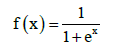
Neural Network: Biological neuron and its simplified features serve as the basic unit of artificial neural networks. These were created as a simplified mathematical model simulating operation of the human brain [6]. It consist of n inputs creating vector x=(x1, .....xn). Each input is multiplied by the corresponding weight parameter, which can be positive or negative. Another input neuron x0=1 is rated by weight x0, which represent the bias [1]. A simple neuron model shown in Figure 1.
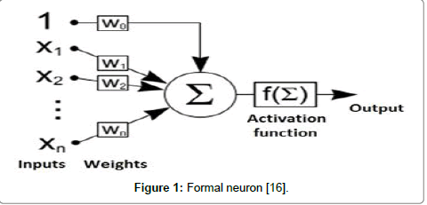
Figure 1: Formal neuron [16].
The sum of all weighted inputs yin indicates the internal potential of the neuron:
 (1)
(1)
The weighted sum is passed through a neuron activation function y = f (y_in) and produce the final output of the neuron. Which turn can become stimulus for neurons in the next neural network layer. The simplest type of activation function is threshold function:
 (2)
(2)
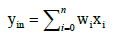
This simple model of neuron is known as perceptron [7]. The interconnection of neurons create neural network. Connection method is such that the output from one neuron is the input of other neurons [1]. Neurons in the network are organized into layers (Figure 2). Each network includes input, output layer and any number of hidden layers [7]. An important feature of neural network is to change the weights between neurons. The weights in the network are strengthened or weakened, depending on the right or wrong answers. There are three types of learning algorithm such as supervised, unsupervised and reinforcement [1,7]. Multilayer perceptron is multilayer neural network in which each neuron is modeled as a perceptron. Activation functions of neurons in multilayer perceptron is differentiable continuous function, most used is a sigmoid function [8]:
Figure 2: Example of a neural network; freely adapted from Volna [1].
 (3)
(3)
Multilayer perceptron lead to the full interconnection of neurons - each neuron in the layer is connected to all the neurons of the above (following) layer.
MLP are the most popular type of neural networks used recently. They belong to a general class of structures so-called feed forward neural networks and present a very basic type of neural network.
Back-propagation algorithm: The MLP is trained using backpropagation algorithm. This is a supervised learning and it takes two stages. First is the feed-forward propagation. The second phase is backpropagation. For each neuron in input layer is calculated gradient of the error function at each iteration step, which is the part of error transmitted to the left of the unit (to previous layer) according to formula:
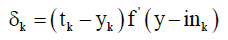 (4)
(4)
Where tk is the expected output of neuron, yk is the calculated output and y_ink is the internal potential of a neuron Yk. Than to each neuron Zj in the inner layer is assigned sum δk from output layer:
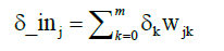 (5)
(5)
With this sum and the derivative of the internal potential z_inj of neuron zj is calculated partial error δj
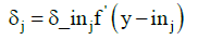 (6)
(6)
Calculated δj is used to adjust the weights between input and internal layer of the network: Δvij=αδjxi, where α is the coefficient of learning and xi is the input value of the network. With δk are adjusted weights between inner and output layer of the network: Δwjk=αδkzj. where zj is the value of the output from neuron Zj. Next, the weighs on connections between neurons are updated. New weight is denoted as n and old as s. Than vij(n)=vij(s)+Δvij and wjk(n)=wjk(s)+Δwjk
Topology of neural networks: First several MLP neural networks with different number of neurons in hidden layers were created. Then trained on training dataset using back propagation algorithm and tested on smaller (testing) dataset, which was not used while training. The mean square error (RMSE) was calculated from trained MLP on test data and few of the best MLP configurations were selected for later calculations.
Custom Interpolation: Using three distinct datasets representing terrain with different characteristics, the interpolation was performed in software’s GRASS 6.4 and R. The interpolation method IDW, krigig and MLP were used. Interpolation was done for each simulated terrain. In software GRASS 6.4; 12 raster’s were created while analysis (three from MLP trained on raster data, six from MLP trained on vector data and three from IDW); in R software; 12 raster’s were created (six by MLP from each package (nnet and neuralnet), six by methods IDW and simple kriging).
Evaluation results of interpolation: For all interpolation results was calculated RMSE according to formula:
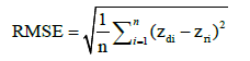 (7)
(7)
Where n is number of points, zdi is the value of point i; zri is the real value in this point. In order to visually compare applied methods, results were subtracted and the difference between them was calculated. Each time raster created by IDW and simple kriging was subtracted from raster generated MLP.
GRASS 6.4
Works with feed forward neural networks; trained with the backpropagation algorithm using 5 scripts written in Python programming language invoking Fast Artificial Neural Network (FANN) library [9]. This script works with raster data. Scripts and their functions are: ann. create creates ANN define file; ann.info displays information about defined ANN; ann.data.rast prepare the learning datasets using raster layer data. ann. learn perform learning and ann.run.rast run the trained ANN to create output raster layer (Netzel) [9].
R project
The R Project software work with feed forward ANN by nnet and neuralnet packages.
The nnet package [10] allow for training feed forward networks by back-propagation algorithm. This network has only one hidden layer. The possible setting parameters are: the number of input and desired output of neurons, number of neurons in hidden layer, weight parameter and maximum number of epoch. Learning of the network is relatively fast and the quality of the result is comparable with other methods.
The neuralnet package [11] in many respects resemble nnet package, but provide more setting parameters. In opposition to the previous package, it is possible to design more than one hidden layer with any number of neurons; additionally user can choose between few available learning algorithms as well as activation function. The training of network is slower than in case of nnet package, but resulting total error is usually smaller.
Inverse Distance Weighting (IDW)
IDW or method of inverse distance weighting is one of the most popular interpolation methods. It is relatively simple in implementation. IDW belongs to exact interpolation method; which do not change measured known values while computation [12]. This method estimate unknown values as average weight of the surrounding known values, in condition that values which are closer have higher weight than those farther away. The value of an unknown point is calculated using following formula:
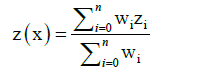 (8)
(8)
Where z(x) is unknown value v in point x, zi are known value and wi are their weight [12].
There are several ways to determine the weight of points with known value. Most often used is the one in which the weight are calculated as the reciprocal value of the distance from point with an unknown value and distance d to the power p [13].
 (9)
(9)
It is recommended to set parameter p in range 1 – 3. If p < 1 then result of interpolation is less flatted. When p > 1; then vice versa [14]. Selection of points with known value from which the unknown value will be calculated can be done in several ways. Most often the number of nearest points involved in calculation is determined another option to set the threshold distance, behind which points have no effect on the calculation [13].
IDW method has characteristic undesirable phenomena that arise as a result of the calculation of average weights. The method of calculation allows the creation of new values only in the range of existing values. If interpolated terrain directed by peaks and valleys, then peaks will appear as depressions and vice versa [12]. Another undesirable phenomenon is the formation of concentric contour lines around points, with the initial value called bull’s eyes [13]. IDW method is readily available in most GIS software such as ArcGIS, QGIS, GRASS GIS, IDRISI, and R (Figure 3).
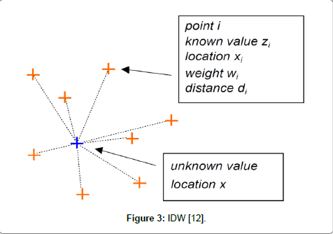
Figure 3: IDW [12].
Ordinary kriging
The basic idea behind kriging is to find certain general characteristics from measured value and applying these properties, when calculating the unknown value. From these properties the most important is smoothness. Theory says that the values in close location to searched point are more similar than in more distant points. The difference of values z between two points is calculated as:
(z(x)) - z(xi))2(10)
With increasing distance between points, it is probable that value z will be also increasing until certain distance and then it will not change [12]. Figure 4 is an example of semivariogram that illustrates how the differences in pairs of points from the measured values change. Sill indicates the maximum value the semivariogram, attains range describes the lag at which the semivariogram reaches the sill. The value of semivariance is never 0, even zero distance. Therefore the parameter nugget indicates the value of difference between two points in the same site, or at a very small distance. Crosses indicate the difference between selected pairs of points; wheels are averages of these values at a certain distance [12]. Ordinary kriging is standard and frequently used version of kriging. Value z in point so is calculated by following formula:
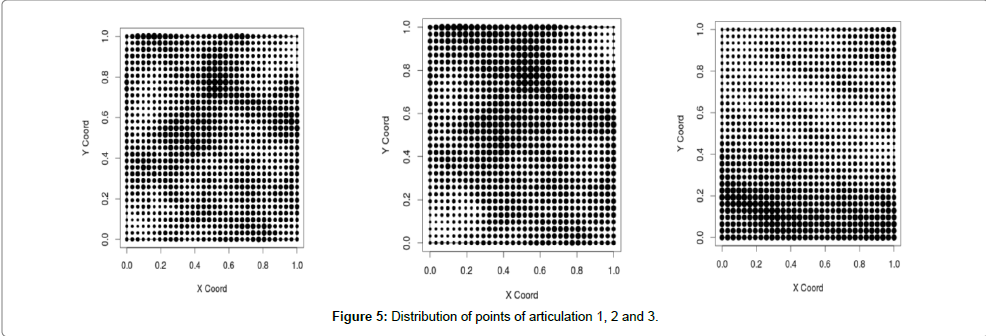
Figure 4: Example semivariogram [12].
 (11)
(11)
Where n is the number of points used in calculations, wi is a weight for point z(s0) and z(si) is a point with known value z. In short, therefore λ0 is the vector of weight wi and z is the vector of n points of known values. Weight wi are calculated using the system of equations [15]. As IDW, simple kriging interpolation method is known and available in the popular GIS software.
Creating data
To provide interpolation using MLP. Three artificial datasets were created in R Project. The dataset simulate different roughness of the terrain. The model with higher roughness was signed as 1, with less roughness as 3. The datasets were randomly generated using function GRF (Gaussian random fields) from package geoR that create points and randomly assign values to them. These values are influenced by other parameters of the function.
grf(pocetBodu, grid=”reg”, cov.pars=c(sill, range), nug=nugget, cov.model=cov Model, aniso.pars=c(anisotropy Direction, anisotropy Ratio), xlims = xlims, ylims = ylims)
Parameter grid=”reg” indicate that points are generated in a regular grid. Parameter cov.model determines the type of variogram, here spherical. Values xlim and ylim were set in interval 0 - 1. There were 1024 points generated in a regular grid for each dataset. These points had three attributes: coordinates x and y from range 0 – 1 and value z which represented elevation. Parameters value describing roughness, used while creation of datasets is given in Table 1.
| Sill | Range | Nugget | Anisotropy ratio | |
| Roughness 1 | 0.12 | 0.3 | 0.00001 | 0.8 |
| Roughness 2 | 0.08 | 0.5 | 0.00001 | 0.8 |
| Roughness 3 | 0.01 | 1.2 | 0.00001 | 0.3 |
Table 1: Parameter values for all surface contours.
Figure 5 is shown in the distribution of points in different datasets. Larger diameter wheels indicate higher z. Training data consist of 724 randomly selected points and was used for learning MLP. Test data contained remaining 300 points and were used to calculate RMSE.

Figure 5: Distribution of points of articulation 1, 2 and 3.
Selecting optimal configuration of MLP using nnet package
The configuration of MLP was determined using test-and-trial method. To make the work more effective, a script gradually creating datasets for all surface topography was created. For each roughness of terrain 10 datasets were created and these datasets were divided into training and testing part. In next step 10 MLP was learned using training data from each existing datasets. Later, for all testing sets RMSE was calculated. This procedure was carried out a total of fifteen times, each time through the varied number of neurons in hidden layer in the range 15 to 30. For each roughness RMSE was calculated. In the last step average RMSE was calculated for all roughness for each MLP configuration. Results are listed in Table 2. Best setting is found MLP with 28 neurons in the hidden layer. Selecting optimal configuration of MLP using neuralnet package: this is similar to nnet package. The difference is that neuralnet package allows trained networks with more hidden layers. Gradually networks were tested with one to four hidden layers. The number of neurons in the first hidden layer is always moved in the interval of 15 to 30. The number of neurons in other hidden layers has been fixed and was selected from a number of 5, 10, 15, 20, and 25. Average RMSE test set was again calculated for all datasets. 24, 15, 10, 5 number of neurons were selected as the best network with four hidden layers. Results of testing networks are in Table 3.
| Number of neurons | Articulation 1 | Articulation 2 | Articulation 3 | Segmentation average |
| 28 | 0.148758 | 0.096397 | 0.017947 | 0.087701 |
| 24 | 0.151135 | 0.096007 | 0.018192 | 0.088444 |
| 25 | 0.149176 | 0.099806 | 0.018237 | 0.089073 |
| 26 | 0.154605 | 0.095057 | 0.017955 | 0.089206 |
| 22 | 0.152875 | 0.097339 | 0.018894 | 0.089703 |
| 30 | 0.157484 | 0.095408 | 0.018022 | 0.090304 |
| 19 | 0.154560 | 0.097975 | 0.018826 | 0.090454 |
| 20 | 0.157060 | 0.097911 | 0.018621 | 0.091197 |
| 18 | 0.156477 | 0.098647 | 0.019657 | 0.091594 |
| 29 | 0.163756 | 0.095861 | 0.018037 | 0.092551 |
| 21 | 0.161621 | 0.097511 | 0.019381 | 0.092838 |
| 16 | 0.161058 | 0.099874 | 0.019209 | 0.093380 |
| 23 | 0.167908 | 0.095541 | 0.019640 | 0.094363 |
| 27 | 0.158991 | 0.106556 | 0.018620 | 0.094722 |
| 17 | 0.166058 | 0.100206 | 0.019149 | 0.095138 |
| 15 | 0.164467 | 0.103390 | 0.019708 | 0.095855 |
Table 2: Average RMSE for testing network setting (nnet).
Selecting optimal configuration of MLP using GRASS 6.4
| Number of neurons | Articulation 1 | Articulation 2 | Articulation 3 | Segmentation average |
| 24 | 0.149159 | 0.098706 | 0.029940 | 0.092602 |
| 16 | 0.153596 | 0.098004 | 0.029210 | 0.093603 |
| 15 | 0.148941 | 0.100402 | 0.032237 | 0.093860 |
| 22 | 0.150838 | 0.097616 | 0.033587 | 0.094014 |
| 20 | 0.149615 | 0.098070 | 0.035774 | 0.094486 |
| 30 | 0.150110 | 0.098537 | 0.035594 | 0.094747 |
| 17 | 0.152036 | 0.100431 | 0.031792 | 0.094753 |
| 23 | 0.152735 | 0.099836 | 0.031717 | 0.094763 |
| 27 | 0.155015 | 0.096519 | 0.033971 | 0.095169 |
| 29 | 0.150820 | 0.098389 | 0.036693 | 0.095301 |
| 26 | 0.152207 | 0.099028 | 0.034765 | 0.095333 |
| 28 | 0.151465 | 0.098248 | 0.038276 | 0.095996 |
| 21 | 0.153177 | 0.099907 | 0.036171 | 0.096418 |
| 19 | 0.150610 | 0.102501 | 0.036541 | 0.096551 |
| 18 | 0.152551 | 0.101085 | 0.038194 | 0.097277 |
| 25 | 0.156908 | 0.101286 | 0.033683 | 0.097292 |
Table 3: Average RMSE for testing network settings (neuralnet).
The module ANN allows training network with multiple hidden layers. As well as in previous methods, an optimal configuration for MLP was found using test-and-trial method. The network with three hidden layers and the number of neurons 32, 38, 27 was selected as most successful MLP setting.
IDW
This method is implementer in R Project software in several packages; in this work gstat package was used with the function idw.
idw_result <- idw (z~x+y=train.set locations, New Data=grid, nmax=18, idp=1.0
Function idw use parameter formula to distinguish coordinates and values which will interpolated. Parameter locations define data used for interpolation and newdata parameter specifies the new coordinates. Number of points that are used in interpolation is set with the parameter nmax (the chosen is 18). Number p (power) is specified in parameter idp.
Kriging
The method of kriging is implemented very extensively in R Project – there are plenty of packages and functions available. From purposes of this work package automap with function auto Krige was used because it allows for ordinary kriging. To generate variogram function autofit Variogram was used.
variogram <- autofitVariogram(z~1, train.set, model = cModel)
kriging_result <- autoKrige(z~1, train.set, grid, model = cModel)
Variogram type specified for interpolation was selected as spherical because artificial data used for interpolation was created in base of spherical variogram. The output of the function autoKrige is Spatial Points Data Frame object, which contained both results and data variogram setting and other things that should not be used in this work. Therefore, the variable b was created which contained the results: coordinates the result of interpolation, variance and standard deviation. As the final result only coordinates and interpolation output was stored.
Calculation of RMSE and visual comparison
To assess the quality RMSE was calculated and compare tested interpolation methods. Assessment was carried out in R Project. When estimating RMSE for surfaces interpolated in GRASS 6.4 from raster data, the vector layer of randomly located points was created by command v.random. To this points the value of original and interpolated raster were added. After these preparations, the data were exported to SCV format using command v.out.ogr. In the next step, the CSV file was imported to R Project where elevation values z were normalized by formula 12 and RMSE was calculated. When estimating RMSE for surfaces interpolated in GRASS 6.4 from vector data, at first the points from test.set were imported to GRASS 6.4. Using command v.what.rast the corresponding values from interpolated raster were added. Next, the file with points were imported to R Project, than the normalized values were transformed to real ones using formula 13 and RMSE was calculated. The steps while analyzing outputs from IDW method was analogous but the values after interpolation was real and there was not need to convert it. The calculation of RMSE was carried out in R Project in the same way for each interpolation methods. The RMSE was calculated for interpolation results coming from test data. The interpolation output from MLPs was transformed from normalized to real values according to formula 13. Next, the original values of elevation were added and finally the RMSE was calculated.
Main results are following:
• Assessment of the quality of interpolation using ANN in GRASS GIS 6.4-svn,
• Comparison of ANN module and interpolation method IDW and kriging,
• Comparison of interpolation using neural networks in GRASS GIS and R Project,
Evaluation of the interpolation quality
First interpolation with the neural network trained on raster data was evaluated. RMSE values with decreasing segmentation data (falling range of values z) decreased. Learning time was longer with the increasing number of the vector points. Learning time was shorter with lower segmentation data. The less iterations were required to train the networks when more vector points were used. Table 4 summarizes data about training the neural network.
| Segmentation | Number of points | Time in minutes | Learning iterations | RMSE |
| Segmentation 1 | 500 | 12 | 13292 | 0.099482 |
| 1000 | 22 | 11675 | 0.106778 | |
| 2000 | 25 | 7901 | 0.088307 | |
| 3000 | 39 | 7618 | 0.064648 | |
| Segmentation 2 | 500 | 10 | 10729 | 0.068894 |
| 1000 | 18 | 10014 | 0.056571 | |
| 2000 | 25 | 6998 | 0.039702 | |
| 3000 | 23 | 3903 | 0.042661 | |
| Segmentation 3 | 500 | 4 | 4863 | 0.010265 |
| 1000 | 13 | 9534 | 0.009793 | |
| 2000 | 14 | 3403 | 0.009272 | |
| 3000 | 11 | 1717 | 0.008466 |
Table 4: Network training data for each segmentation.
The range of values z in the interpolated grid is lower than the range of values in the original grid (Table 5). This could be due to poor distribution of random vector points. RMSE value in this case was 0.0646. In case of segmentation 1, neural network has missed extreme values. In segmentation 2, difference in the rage is smaller; which means the random vector points were probably better distributed. However the extreme values are also omitted. The value of RMSE is 0.0427. In case of segmentation 3, network behaviour is similar to the previous two cases and the value of RMSE is 0.0085. The value of RMSE was then expressed in percentage according to the range of value z. The difference between the values of RMSE is only 1%; for each segmentation (Table 5).
| Original data range | Interpolated grid | RMSE % | |
| Segmentation 1 | -0.6924255 - 1.034648 | -0.6198587 to 0.8887726 | 4.2852 |
| Segmentation 2 | -0.5086115 - 0.863945 | -0.4962887 to 0.7969054 | 3.2989 |
| Segmentation 3 | -0.1734903 - 0.124689 | -0.1563402 to 0.1131727 | 3.1412 |
Table 5: Range of value z in original and interpolated data and comparison of RMSE for all segmentation.
Interpolation quality was further evaluated by visual comparison of resulting raster’s. Neural network from ANN module trained on raster data was able to adapt quite well and resulting grid was very similar to the original grid. Figure 6 shows the original and interpolated grid for segmentation 1.
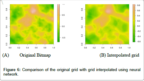
Figure 6: Comparison of the original grid with grid interpolated using neural network.
Figure 7 shows differences in the z values between the new and original grid. Original grid was subtracted from the new grid. Grid created with neural network has z values, usually lower than the original bitmap. The average value of the difference was -0.03145 and highest differences were -0.32560 and 0.18220.
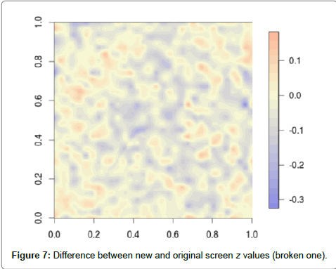
Figure 7: Difference between new and original screen z values (broken one).
Neural network from the ANN module trained on vector data file had a similar behaviour as the network trained on raster data file. It was necessary to change learning coefficient, when training the network on vector data. Table 6 summarizes the data about training the neural network with the numbers of 32, 38, 27 neurons and the neural network with the numbers of 20, 25, 17 neurons for each segmentation.
| learning time in minutes | Iterations learning | Coefficient | RMSE | ||
| Network 32, 38, 27 | Articulation 1 | 42 | 32494 | 0.7 | 0.212881 |
| Articulation 2 | 47 | 36136 | 0.4 | 0.126754 | |
| Articulation 3 | 14 | 3403 | 0.1 | 0.017628 | |
| Network 20, 25, 17 | Articulation 1 | 7 | 10504 | 0.4 | 0.140651 |
| Articulation 2 | 3 | 5021 | 0.4 | 0.098192 | |
| Articulation 3 | 2 | 3104 | 0.4 | 0.025206 |
Table 6: Data on training networks for each segmentation.
During interpolation of the neural network again omitted extreme values. In segmentation 2, the lower boundary of the interval z values in a new grid was lower than in the original data. Range of z values in the original and newly interpolated data can be found in Table 7. Which show values for a grid created with neural network with the number of 20, 25, 17 neurons. RMSE value was 0.1407 in case of segmentation 1, 0.0982 in segmentation 2 and 0.0252 in case of segmentation 3. These values and percentage are higher than the grid created with network trained on raster data file. In segmentation 3, values are higher as selected network parameters and were not entirely suitable for segmentation of data.
| Original data range | Interpolated grid | RMSE % | |
| Articulation 1 | -0.7396643 - 1.090838 | -0.6786178 to 0.9450067 | 8.6658 |
| Articulation 2 | -0.5203077 - 0.893018 | -0.6193843 to 0.6952054 | 7.4700 |
| Articulation 3 | -0.2012766 - 0.141199 | -0.1532334 to 0.0899525 | 10.3624 |
Table 7: Range of values z original and interpolated data on (20 25 17) network and comparison of RMSE for all segmentations.
Comparison of ANN, IDW and kriging method
The input data selected for input neurons is same as used in IDW and ordinart kriging. The criterion for comparison was RMSE value, time demand and user friendliness.
Comparison by RMSE: Figure 8a compares the RMSE values of resulting raster’s. The network used in this comparison was the one with number of 38, 32, 27 neurons. RMSE values of raster generated by the network were in case of segmentation 1 and 2, higher than value of other two methods. This was due to the wrong setting of network parameters; may be network probably got over-trained. Table 8 is recorded RMSE values with four decimal accuracy places.
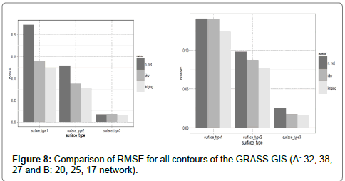
Figure 8: Comparison of RMSE for all contours of the GRASS GIS (A: 32, 38, 27 and B: 20, 25, 17 network).
| n network(32, 38, 27) | IDW | kriging | ||
| n network (32, 38, 27) | articulation 1 | 0.2221 | 0.1398 | 0.1240 |
| articulation 2 | 0.1285 | 0.0874 | 0.0770 | |
| articulation 3 | 0.0172 | 0.0177 | 0.0158 | |
| n network (20, 25, 17) | articulation 1 | 0.1407 | 0.1398 | 0.1240 |
| articulation 2 | 0.0982 | 0.0874 | 0.0770 | |
| articulation 3 | 0.0252 | 0.0177 | 0.0158 |
Table 8: RMSE values for all segmentation for GRASS GIS.
Figure 8b compare all methods, the network used in this comparison is one with number of 20, 25, 17 neurons. In this case RMSE values were comparable for all methods, but in case of segmentation 2 and 3; values of RMSE for raster interpolated using neural network were higher. This was probably caused by network parameter settings that did not fit the data from this segmentation. Table 8 records the RMSE values with accuracy of four decimal places.
The RMSE value of raster’s interpolated by neural networks were higher than the values of raster created by IDW and kriging. Although it was assumed that neural networks would have better results. There are several reasons: Despite the testing of neural networks settings. It is possible that inappropriate parameters were chosen to fit the nature of data and networks were trained poorly. The other reason for worse results of the neural networks might be insufficient number of input parameters – only two were used. Figure 9 shows comparison of the RMSE value for all methods in R Project. RMSE values of raster’s by neural networks from both packages were higher than values of raster’s by IDW and kriging methods.
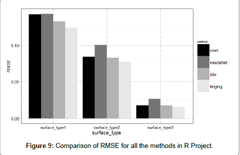
Figure 9: Comparison of RMSE for all the methods in R Project.
RMSE values for the nnet package for segmentation 2 and 3 are most similar to the RMSE value for the other methods. Table 9 shows the RMSE values with an accuracy of four decimal places. Figure 10 shows the resulting raster interpolated with neural networks, IDW and kriging in GRASS GIS for the segmentation 1.
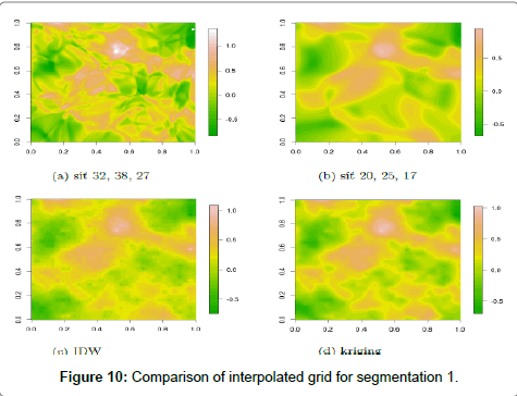
Figure 10: Comparison of interpolated grid for segmentation 1.
| nnet | NeuralNet | IDW | Kriging | |
| Articulation 1 | 0.1418 | 0.1427 | 0.1325 | 0.1240 |
| Articulation 2 | 0.0843 | 0.1002 | 0.0828 | 0.0770 |
| Articulation 3 | 0.0177 | 0.0264 | 0.0176 | 0.0158 |
Table 9: RMSE values for all the contours of the R Project.
Figure 11 show the differential bitmap for segmentation 1. Figures 11a and 11b show the difference in z values between raster’s created by neural network (32, 38, and 27) and other methods. Maximum values of difference between the network and the IDW were -0.784100 and 0.707100 and the average value was 0.006563. Values in raster interpolated using IDW was therefore lower than the values in raster interpolated using neural networks. Maximal value of difference between the network and kriging were -0.666400 and 0.686100 and average value was 0.005321. Values in raster interpolated using kriging were also a bit lower than the values in raster interpolated using neural networks.
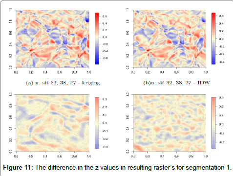
Figure 11: The difference in the z values in resulting raster’s for segmentation 1.
Figures 11c and 11d show the differences in z values between raster’s created by neural network (20, 25, and 17) and other methods. The maximum value difference between the network and IDW were -0.3207000 and 0.3265000 and average value was 0.0030340. Maximal value of difference between the network and kriging were -0.272800 and 0.305600. The average value difference was -0.001977. Raster created by IDW and kriging methods has higher values. The differences between this network, IDW and kriging method is lower than in the first case.
Comparison by time-consuming: The time required to perform an interpolation is shown in Table 10. These values in case of neural networks include the time needed to train the network and time required to perform the calculation. In case of other methods, only time required to perform the computation is shown. A neural network is time consuming due to the long training time. If wrong parameters were chosen; then training took a very long time (Table 10). With the better parameters, training time was distinctively shorter. With decreasing segmentation of the data the training time decreased as well. Calculation time was very short; once the networks were properly trained. Segmentation of the data did not affect the speed of calculation; in any method. The longest computation time had the kriging. The fastest interpolation method was IDW. Interpolation with the neural network was the longest one, mainly because of the time needed to train the networks.
| n network (32, 38, 27) | n network (20, 25, 17) | kriging | IDW | |
| articulation 1 | 42 | 7 | 3 | 0.5 |
| articulation 2 | 47 | 3 | 3 | 0.5 |
| articulation 3 | 14 | 2 | 3 | 0.5 |
Table 10: Time required to performing interpolation (in minutes).
Comparison by the user friendliness: This review summarizes the work with availability methods to help and comprehensibility of used methods. IDW method and script v.surf.idw is part of the main installation of GRASS GIS. It can be used via the command line or the graphical interface. When working in the graphical interface a manual is available. It describes each setting that, what is the affect when used and in the last a short theoretical summary. Kriging method does not exist as a module in GRASS GIS. It can be used by connecting the GRASS GIS with R Project program. Only the command line is available for the user. Manual and instructions how to work with the kriging method is available in the R Project as well as in the internet. The ANN module is not a part of main installation of GRASS GIS and it`s not stored in the repository modules accessible via the command g.extension. It can be downloaded from http://grasswiki.osgeo.org/wiki/AddOns web page. The ANN module can be operated both in command line and graphical interface, but manual is not included. It has to be opened separately. The manual describes necessary values for parameters but the effect to the outcomes is not mentioned. Unlike the IDW or kriging method, the use of ANN module is difficult for inexperienced users due to lack of knowledge of neural network. A brief manual is not too useful.
Comparison of interpolation using neural networks in programs GRASS GIS and R Project: Comparisons were carried out in several respects. When compared by RMSE there was no significant difference between the neural networks from GRASS GIS and R Project. Figure 12 compare the values of RMSE for the two networks from the GRASS GIS, nnet and neuralnet package. For segmentation 1, values were almost equal, except the network (32, 38, and 27) of GRASS GIS, which was probably over-trained. This also happened in case of segmentation 2. Values of RMSE for other networks were again similar and best results were given by the nnet package. In case of the segmentation 3; values were again quite similar for (20, 25, and 17) network. Network of neuralnet package showed signs of over-training. The best results for this segmentation were given by the network (32, 38, and 27) from GRASS GIS. Used neural networks in both programs were chosen as one of the best possible for the available data. RMSE values for each segmentation is not much different. If the neural networks with different parameters were used. Results would have probably differed more or less. Table 11 is recorded RMSE values from Figure 12.
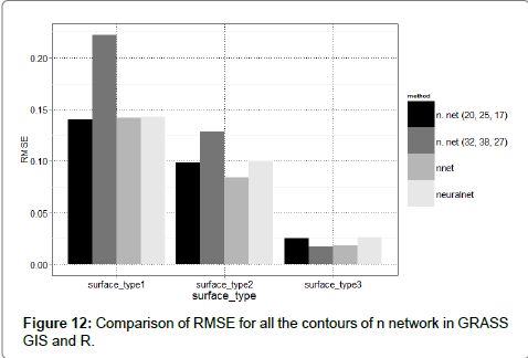
Figure 12: Comparison of RMSE for all the contours of n network in GRASS GIS and R.
| n network (20, 25, 17) | n network (32, 38, 27) | nnet | neuralnet | |
| Articulation 1 | 0.1407 | 0.2221 | 0.1418 | 0.1427 |
| Articulation 2 | 0.0982 | 0.1285 | 0.0843 | 0.1002 |
| Articulation 3 | 0.0252 | 0.0172 | 0.0177 | 0.0264 |
Table 11: RMSE values for all segmentation for GRASS GIS and R Project.
The training speed of the networks in ANN module and R Project depends primarily on the number of neurons in the hidden layers, the segmentation of input data and size of training dataset. In case of the ANN module it also depends on appropriate parameter settings.
However the neural network packages in R Project train faster than the networks in the ANN module. Figure 13 shows the resulting bitmaps of the neural network for segmentation 1. The resulting raster in partial Figures 13a, 13b and 13d are visually quite similar and RMSE values is not much differ. Resulting raster in sub Figure 13c differ significantly both in visually and RMSE value.
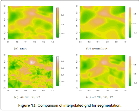
Figure 13: Comparison of interpolated grid for segmentation.
Evaluation and testing results shown that neural networks in GRASS GIS can be used for spatial interpolation, but it`s (MPL) not better than IDW and kriging method. The disadvantage of ANN module is work with raster data only (in present version), but the interpolation from vector data. Without the user intervention (in this research work using a custom script that transformed vector data in the desired format) the ANN module is not very useful for normal interpolation. After comparing the neural networks from both software’s for the purpose of normal interpolation the R Project is better than GRASS GIS, although neither network in the R Project had better results than the methods IDW and kriging. The use of multilayer perceptron for spatial interpolation is an interesting option to classical methods. Bur it’s requiring more knowledge of theory from the user and time consuming. The results are often uncertain and the training of MLP has to be repeated many times to reach satisfactory results. The ANN module is in its current form cannot yet be regarded as equivalent to the conventional methods; however future development of this module might make a difference.