Drug Designing: Open Access
Open Access
ISSN: 2169-0138
ISSN: 2169-0138
Review Article - (2014) Volume 3, Issue 2
In recent years, the concept of quality by design in (global) pharmaceutical development has received much attention. The purpose is to ensure that the compound under investigation will possess good drug characteristics such as identity, strength, purity, quality, safety, efficacy and stability before and post approval. A pharmaceutical development process consists of non-clinical (e.g., assay/process validation and stability testing), pre-clinical (e.g., animal and bioavailability/bioequivalence studies), and clinical (e.g., phases 1-3 clinical trials) development. In this article, various statistical designs that are commonly considered for achieving desired good drug characteristics as described in the United States Pharmacopeia and National Formulary (USP/NF) at various stages of non-clinical, pre-clinical, and clinical development are reviewed. In addition, the possible use of innovative adaptive clinical trial designs that may lead to (i) the identification of any signals, trends/patterns, and optimal clinical benefits of a test treatment under investigation, and (ii) increase the probability of success of the development process with limited resources available are discussed.
<Keywords: Pharmaceutical development process, Quality by design, Assay validation, Process validation, Stability analysis, Adaptive design methods in clinical trials
In the pharmaceutical industry, the ultimate goal of a pharmaceutical development process is to produce high quality, safe and efficacious drug products for human use. The pharmaceutical development process, involving drug discovery, formulation, laboratory development, animal studies, clinical development, and regulatory registration, is a continual, length, and costly process. This lengthy and costly process is necessary to assure the safety and efficacy of the drug product under investigation. After the drug is approved, the United States Food and Drug Administration (FDA) also requires that the drug product be tested for identity, strength (potency), quality, purity, and stability before it can be released for human use.
Basically, a pharmaceutical development process consists of different phases of development, including non-clinical development (e.g., assay development/validation in laboratory development, manufacturing process validation, and stability testing and analysis), pre-clinical development (e.g., animal studies and bioavailability/ bioequivalence studies), and clinical development (e.g., phase 1-3 clinical development) [1]. These phases may occur in sequential order or be overlapped during development process. At different phases of pharmaceutical development, valid statistical designs are usually employed to ensure that the drug product possesses good drug characteristics such as identity, strength, quality, purity, safety, efficacy, and stability before and post-approval of the drug product.
In this article, we will not only introduce the concept of quality by design suggested by the FDA, but also provide an overview of statistical designs that are commonly employed at different phases (stages) of a pharmaceutical development. In addition, the potential use of various adaptive trial designs in clinical development for not only shortening the development process but also for increasing the probability of success of the development process with limited resources available is also discussed.
In the next section, the concept of quality by design recommended by the FDA [2,3] is briefly introduced. Statistical designs that are commonly employed in non-clinical, pre-clinical, and clinical development are reviewed in Nonclinical Application, Pre-clinical Application, Clinical Application. Also included in Clinical Application is some discussion of the potential use of adaptive designs in clinical trials. A brief concluding remark is given in the last section of this article.
In the pharmaceutical industry, it is recognized that reasonable high quality product can only be achieved at a great effort and cost. In practice, pharmaceutical companies mainly focus on development rather than put their emphasis on manufacturing. In many cases, the manufacturing process is not only unable to meet pre-specified quality standard, but also inability to predict effects scale-up on final product. Quality by design is a concept that quality could be planned, and that most quality crises and problems relate to the way in which quality was planned. In recent years, FDA has considered quality by design as a vehicle for the transformation of how drugs are discovered, developed, and commercially manufactured. In the past few years, the FDA has implemented the concepts of QbD into its pre-market processes. The focus of this concept is that quality should be built into a product with an understanding of the product and process by which it is developed and manufactured along with a knowledge of the risks involved in manufacturing the product and how best to mitigate those risks. This is a successor to the “quality by QC” (or “quality after design”) approach that the companies have taken up until 1990s. Winkle [2] provides a comprehensive comparison of traditional approach with the systematic QbD approach (see Table 1). For example, under the concept of QbD, decisions are made based on scientific findings rather than empirical ones. To determine whether the test product possesses good drug characteristics such as identity, strength, purity and quality, unlike the traditional approach, it is suggested that multivariate experiments should be performed to make sure that the test product meets product specifications (e.g., as described in USP/NF, 2000). For development and validation of manufacturing process, traditional approach is to test whether each performance characteristics such as potency (% of label claim) meet specific product specification by ignoring the fact that these performance characteristics may be related. One disadvantage of this fixed approach is that some key performance characteristics may meet specific specifications but some don’t. With appropriate adjustable, we will be able to meet specific product specification for each performance characteristics and at the same achieve desirable (optimal) quality of the manufacturing process.
| Aspects | Traditional | Quality by Design |
|---|---|---|
| Pharmaceutical Development | Empirical; Univariate experiments |
Systematic; Multivariate experiments |
| Manufacturing Process | Fixed | Adjustable |
| Process Control | In-process testing for go/no-go; Offline analysis w/slow response |
PAT utilized for feedback and feed forward at real time |
| Product Specification | Primary means of quality control; Based on batch data |
Overall quality control strategy; Based on desired product performance (safety and efficacy) |
| Control Strategy | Based on intermediate and end product testing |
Risk-based; Controls shifted upstream; Real-time release upstream |
| Lifecycle Management | Reactive to problems; Scale-up and post-approval changes |
Continual improvement enabled within design space |
Note: PAT=Process Analytical Technology
Modified from Winkle [2].
Table 1: A Comparison between Traditional Approach and QbD Systematic Approach.
Winkle [2] pointed out that the implementation of quality by design is not only beneficial to industry but also to FDA. As an example, from the perspectives of pharmaceutical industry, quality by design ensures the production of better products with fewer problems in manufacturing. The use of quality by design cannot only reduce number of manufacturing supplements required for post market changes and at the same time, allow for implementation of new technology to improve manufacturing without regulatory scrutiny. In addition, it can also improve interaction with FDA reviewers and consequently speed up the review/approval process. On the other hand, from the perspectives of FDA, the implementation of quality by design will not only enhance scientific foundation for review, but also provides better coordination across review, compliance and inspection divisions within the FDA. Second, it not only improves information in regulatory submissions and quality of review, but also provides for better consistency and for more flexibility in decision making. Moreover, it ensures decisions made on science and not on empirical information. Quality by design not only involves various disciplines in decision making, but also allows the FDA to use limited resources to address higher risks more efficiently.
Assay validation
The major objective of the validation of an assay method is to ensure that the assay method can produce unbiased and precise assay results for the active ingredient of a compound. To achieve this objective, a so-called recovery study is usually conducted. The USP/NF indicates that the assay method needs to be validated in terms of the primary validation parameters given in Table 2 (USP/NF 2000). See, also NCCLS (National Committee for Clinical Laboratory Standards) guidelines for validation. To meet the USP/NF standards for each of these parameters, an appropriate statistical design is necessarily chosen to provide sound statistical inferences for these parameters and their variances. In this section, several commonly employed designs in assay validation are briefly described.
| Accuracy | Selectivity |
|---|---|
| Precision | Range |
| Limit of detection (LOD) | Linearity |
| Limit of quantitation (LOQ) | Ruggedness |
Table 2: Performance Characteristics in Assay Validation.
Randomized block design: The randomized block design is probably the most commonly used design in assay validation. Suppose that there are J levels of potency (expressed as percent of label claim) in a recovery study. Samples are usually assayed on different days (say 3 different days) with and/or without the same number of replicates (say 3-5 replicates). Note that J is usually an odd number such as (L, M, H) or (L, L, M, H, H), where L and H indicate below and above of the level of 100% of label claim. This design provides independent estimates of day-to-day variability and within-day variability.
Latin square type of design: In the above design, assays of different levels on the same day are usually performed in sequential order, which may introduce bias due to testing order. To avoid the bias that may be introduced by testing order, it is suggested that a Latin square type of design be used to balance the potential bias. In other words, the number of days should be equal to the number of levels. The Latin square design is then applied to the test sequence of the levels of potency.
Incomplete block design: In practice, the number of assays performed on each day may not be able to cover all the levels of potency under study due to limited resources available. In addition, in some cases, the assay can only be conducted on a certain number of days, which are fewer than the number of levels of potency. In these situations, an incomplete block design may be used to randomize test sequences on each day.
Remarks: For validation of an assay method, recovery studies are conducted not only to estimate the accuracy, linearity, and precision but also to provide statistical inference on the ruggedness across different days or laboratories. Based on the nature of the various purposes of a recovery study, sample size determination has become a challenge to statisticians.
Process validation
A manufacturing process is a continuous process that involves a number of critical stages for quality assurance. For example, for tablets manufacturing process of a pharmaceutical compound, critical stages include active pre-blending stage, the primary blending stage, the lubricant pre-blending stage, the final blending stage, and the compression stage. At each critical stage, problems may occur during the process. For example, the ingredients may not be uniformly mixed at the primary blending stage; the segregation may occur at the final blending stage; a significant loss of active ingredient may encounter during the transfer from the V-blender to the transport devices. Thus, process validation is essential not only to ensure that the process does what it purports to do, but also to ensure that the drug product will conform to USP/NF specifications of good drug characteristics such identity, strength, quality and purity.
Regulatory requirement: In its recent guidance on process validation, FDA emphasizes the concept of quality by design in process validation and notes the need for pharmaceutical companies to continue benefiting from knowledge gained, and continually improve throughout the process lifecycle by making adaptations to assure root causes of manufacturing problems are corrected. For a prospective validation, FDA generally requires that at least three batches be evaluated. For each batch, data are usually collected at each critical stages of the manufacturing process according to a validation design as described in the validation protocol. In practice, a validation design clearly outlines sampling plan, testing plan, and acceptance criteria for validation, which are briefly described below.
Sampling plan, testing plan, and acceptance criteria: The validation of a manufacturing process requires satisfactory results at each critical stage during a manufacturing process for three batches. For each batch, however, sampling plan may be different from stage to stage. For example, at the primary blending stage, twelve 5 g representative samples are usually drawn, one each from the top, middle, and bottom of the front and back from the right and left side of the V-blender after blending for 50, 60, and 70 minutes with the intensifier bar running. At compression stage, 200 tablets are usually removed at the beginning and after each one-ninth by weight of the contents of the transport device as compressed for the first, fourth (middle), and last transport devices emptied from the V-blender. For each batch, testing procedure may be different from stage to stage. For example, at the primary blending stage, for the first batch, 36 samples are used, testing one tablet equivalent per 5 g sample (12 samples per blending time×3 blending times). For the second and third batches, 12 samples (from each batch) are used to test one tablet equivalent per 5 g sample. Thus, a total of 60 samples are tested for three batches. At compression stage, testing plan could be (i) for potency, 15 assays (one from the beginning and from the 2/9, 4/9, 2/3, and end sample from each of three transport devices sampled), (ii) for content uniformity, 120 tablets (40 tablets from each point in the sampling plan), and (iii) for dissolution, 18 tablets (6 tablets from each of the three transport devices sampled; 3 tablets each from the beginning and end of each transport device). Acceptance limits for the validation of a manufacturing process are usually designed to be more stringent to assure that the final product will pass USP/NF specifications. Acceptance limits are a set of sample statistics from which a confidence interval for a given parameter is constructed to meet a pre-specified lower probability bound for passing a particular USP test.
Remarks: For the validation of a manufacturing process, at least three batches or lots must be evaluated. If all three batches or lots pass USP tests, the manufacturing process is considered validated. In practice, however, one of the three batches may fail USP tests at some critical stages of the manufacturing process. In this case, the possible causes for the failure should be investigated. An additional batch or lot should be tested after the problem has been identified and corrected.
Scale-up
In the pharmaceutical industry, it is important to ensure that a production batch can meet the USP/NF standards for the identity, strength, quality, and purity of the drug before a batch of the product is released to the market. Thus, scale-up program plays an important role to scale up a laboratory batch to a commercial (production) batch. The purpose of a scale-up program is not only to identify, evaluate, and optimize critical formulation and/or manufacturing process factors of the drug product but also to maximize or minimize excipient ranges. A successful scale-up program can result in an improvement in formulation/process or at least a recommendation on a revised procedure for formulation/process of the drug product. Some commonly employed designs in scale-up experiments are briefly described below.
Factorial design: A full factorial design is a design that consists of all possible different combinations of one level from each factor. If there are lk levels for the kth factor Xk, the corresponding full factorial design is called a general l1l2….lK factorial design. For example, when li=2 (or 3) for all i, the general factorial design is called a 2K (or 3K) factorial design. A 2K (or 3K) factorial design denotes a full factorial design at two levels (or at three levels). In practice, a factorial design is expressed in terms of a number of arrays (or runs) that indicate the levels of each factor. For example, for a typical 24 factorial design, the arrangement of the arrays is given in the following standard order (Table 3). The first column of the design matrix consists of successive minus (-) and plus (+) signs, the second column of successive pairs of (-) and (+) signs, the third column of four (-) signs followed by four (+) signs, and so on. In general, the Kth column consists of 2K-1 (-) signs followed by 2K-1 (+) signs. In this 24 factorial design, there are four factors at two levels, with a total of N=24=16 runs. The two levels of each factor are conventionally denoted by (+) and (-) (they are sometimes denoted by 1 and -1). If a variable is continuous, the two levels, (+) and (-), denoted the high and low levels. If a variable is qualitative, the two levels may denote two different types or the presence and absence of the variable. Each row represents a different combination of one level from each factor. A full factorial design provides estimates not only for main effects but also for interactions with maximum precision. The main effects and interaction effects can easily be obtained using a table of contrast coefficients and/ or Yate’s algorithm Myers [4]; Hicks [5].
| Design matrix | |||||
|---|---|---|---|---|---|
| Run | X1 | X2 | X3 | X4 | Y |
| 1 | - | - | – | - | Y1 |
| 2 | + | - | - | - | Y2 |
| 3 | - | + | - | - | Y3 |
| 4 | + | + | - | - | Y4 |
| 5 | - | - | + | - | Y5 |
| 6 | + | - | + | - | Y6 |
| 7 | - | + | + | - | Y7 |
| 8 | + | + | + | - | Y8 |
| 9 | - | - | - | + | Y9 |
| 10 | + | - | - | + | Y10 |
| 11 | - | + | - | + | Y11 |
| 12 | + | + | - | + | Y12 |
| 13 | - | - | + | + | Y13 |
| 14 | + | - | + | + | Y14 |
| 15 | - | + | + | + | Y15 |
| 16 | + | + | + | + | Y16 |
Table 3: A Full 24 Factorial Design.
Fractional factorial design: A fractional factorial design is a design that consists of s fraction of a full factorial experiment. For example, a  fraction of a 2K factorial design is called a 2K-P fractional factorial design. When P=1, a full factorial design reduces to a one-half factorial design. For a full 24 factorial design, there are 16 effects, including grand average, four main effects, six two-factor interactions, four threefactor interactions, and a single four-factor interaction. The full 24 factorial design contains 16 observations, which provide independent estimates for each of these 16 effects. However, if we consider only a one-half fraction (i.e., only eight observations available), due to limited resources available, it is impossible to obtain 16 independent estimates. For a 24-1 fractional factorial design, the eight observations cannot provide independent estimates for the 16 effects alone but for some confounding effects, such as the sum of a main effect and a three-factor interaction that are confounded with each other. In practice, however, the three-factor or higher-factor interactions are usually negligible (Table 4). In this case, a fractional factorial design is useful in estimating the main effects. In practice, a fractional factorial design is useful when there are many factors to be studied because it is almost impossible to perform a full factorial design even at two levels.
| Design matrix | |||||
|---|---|---|---|---|---|
| Run | X1 | X2 | X3 | X4=X1 X2 X3 | Y |
| 1 | - | - | - | - | Y1 |
| 2 | + | - | - | + | Y2 |
| 3 | - | + | - | + | Y3 |
| 4 | + | + | - | - | Y4 |
| 5 | - | - | + | + | Y5 |
| 6 | + | - | + | - | Y6 |
| 7 | - | + | + | - | Y7 |
| 8 | + | + | + | + | Y8 |
Table 4: A 24-1 Fractional Factorial Design.
Central composite design: A central composite design is a full factorial design or a fractional factorial design augmented by a ± α level at each of the K factors and n central points. The central composite design consists of one center point, eight points on the cube (a 23 factorial arrangement), and six star points. It should be noted that a central composite design with K=2, α=1, and n=1 reduces to a 32 factorial design (Table 5). For a full 2K factorial design, although the design provides independent estimates for the 2K-1 effects, it does not give an estimate of the experimental error unless some runs are repeated. Unlike the full 2K factorial design, the central composite design provides an estimate of the experimental error. The experimental error is usually estimated based on n observations at the central point.
| Run | X1 | X2 | X3 |
| 1 | –1 | –1 | –1 |
| 2 | 1 | –1 | –1 |
| 3 | –1 | 1 | –1 |
| 4 | 1 | 1 | –1 |
| 5 | –1 | –1 | 1 |
| 6 | 1 | –1 | 1 |
| 7 | –1 | 1 | 1 |
| 8 | 1 | 1 | 1 |
| 9 | 0 | 0 | 0 |
| 10 | α | 0 | 0 |
| 11 | – α | 0 | 0 |
| 12 | 0 | α | 0 |
| 13 | 0 | – α | 0 |
| 14 | 0 | 0 | α |
| 15 | 0 | 0 | –α |
Table 5: Central Composite Design for K=3 and n=1.
Remarks: In addition to the factorial design, the fractional factorial design, and the central composite design, other designs such as the classical Plackett and Burman design [6] and the factorial or fractional factorial in randomized block design are also useful in scale-up experiments.
Stability analysis
Regarding study design and sample selection criteria, the ICH Q5C guideline recommends that a bracketing design or a matrixing design be used [7-11]. Samples can then be selected for the stability program on the basis of a matrixing system and/or by bracketing. A bracketing design is a design that only samples on the extremes of certain design factors which are tested at all time points. Stability at the intermediate levels is considered being represented by the stability of the extremes. Bracketing is generally not applicable for drug substances. Bracketing can be applied to studies with multiple strengths of identical or closely related formulation. In this case, only samples on the extremes of certain design factors (e.g., strength, container size, fill) are tested at all time points. A bracketing design can also be applied to studies with the same container closure system with the fill volume and/or the container size varied.
A matrixing design is a statistical design of a stability study that allows different fractions of samples to be tested at different sampling time points [8,11]. Each subset of samples represents the stability of all samples at a given time point. Differences in the samples should be identified as covering different batches, different strengths, and different sizes of the same container closure system. A matrixing design should be balanced such that each combination of a factor is tested to the same extent over the duration of the studies. It should be noted that all samples should be tested at the last time point before the submission of application. For the purpose of illustration, the following examples exhibit matrixing in a long-term stability study for one storage condition: (S1) one-half reduction eliminates one in every two time points (Table 6 of (S2) one-third design eliminates one in every three time points).
| Time-points (months) | 0 | 3 | 6 | 9 | 12 | 18 | 24 | 36 | ||
| strength | S1 | Batch 1 | T | T | T | T | T | T | ||
| Batch 2 | T | T | T | T | T | T | ||||
| Batch 3 | T | T | T | T | T | |||||
| S2 | Batch 1 | T | T | T | T | T | ||||
| Batch 2 | T | T | T | T | T | T | ||||
| Batch 3 | T | T | T | T | T | |||||
Key: T=Sample Tested
Table 6: Example of Matrixing Design-One-half Reduction. “One-Half Reduction”.
Storage Conditions Since stability data are analyzed using a linear regression, the selection of observations that will give the minimum variance for the slope is to take one-half at the beginning of the study and one-half at the end. The beginning of the stability study is usually called t=0. Stability studies are typically done at several different times. In practice, there is no unique best design. Thus, the choice of design must use the fact that analyses will be done after additional data are collected. Nordbrock [8] introduced several designs that are commonly considered in stability studies. These designs are briefly described below.
Basic matrix 2/3 on time design: A complete long-term study for one strength of a dosage form in one package has three batches, with all three tested every 3 months in the first year, every 6 months in the second year, and annually thereafter. Thus if a 36 month shelf life is desired and the complete study is used, each of the three batches is tested at 0, 3, 6, 9, 12, 18, 24, and 36 months. The basic matrix 2/3 on time design has only two of the three batches tested at intermediate time points (other than at times of 0 and 36), as presented in Table 7. If an analysis is to be done after 18 months (e.g., for a registration application), the basic matrix 2/3 on time design can be modified by testing all batches at 18 months.
| Batch | Test times (months) |
|---|---|
| A B C |
0, 3, 9, 12, 24, 36 0, 3, 6, 12, 18, 36 0, 6, 9, 18, 24, 36 |
Table 7: Basic matrix 2/3 on time design.
Matrix 2/3 on time design with multiple packages: The first extension of the basic design is when one strength is packaged into three packages (i.e., when each batch is packaged into each of three packages). The basic matrix 2/3 on time design is applied to each package in a balanced fashion, as presented in Tables 8 and 9. Balance is defined as testing each batch twice at each intermediate time point, and each package twice at each intermediate time point. If an analysis will be done after 18 months (e.g., for a registration application), this design can be modified by testing all batch-by-package combinations at 18 months.
| Batch | Pkg1 | Pkg2 | Pkg3 |
|---|---|---|---|
| A | T1 | T2 | T3 |
| B | T2 | T3 | T1 |
| C | T3 | T1 | T2 |
Note: Pkg1=Package 1, etc.
Table 8: Matrix 2/3 on Time Design with Multiple Packages.
| Code | Test times after time 0 |
|---|---|
| T1 T2 T3 |
3, 9, 12, 24, 36 3, 6, 12, 18, 36 6, 9, 18, 24, 36 |
Note: Batches are tested at time 0.
Table 9: Test Time Intervals.
Matrix 2/3 on time design with multiple packages and multiple strengths: When three strengths (say, 10 mg, 20 mg, and 30 mg) are manufactured using different weights of the same formulation, nine sub-batches result. We further assume that there are three packages for each strength. In this case, the basic matrix 2/3 on time design can be applied to each of the nine sub-batches in a balanced fashion (Table 10). In this design, each sub-batch is tested twice at each intermediate time point, each package is tested twice at each intermediate time point for each batch, each batch is tested six times at each intermediate time point, and each package is tested six times at each intermediate time point. If an analysis will be done after 18 months (e.g., for a registration application), this design can be modified by testing all batch-bystrength- by-package combinations at 18 months.
| Batch | Strength | Package 1 | Package 2 | Package 3 |
|---|---|---|---|---|
| A | 10 | T1 | T2 | T3 |
| A | 20 | T2 | T3 | T1 |
| A | 30 | T3 | T1 | T2 |
| B | 10 | T2 | T3 | T1 |
| B | 20 | T3 | T1 | T2 |
| B | 30 | T1 | T2 | T3 |
| C | 10 | T3 | T1 | T2 |
| C | 20 | T1 | T2 | T3 |
| C | 30 | T2 | T3 | T1 |
Table 10: Matrix 2/3 on time design with multiple packages and multiple strengths.
Matrix 1/3 on time design: A further reduction in the amount of testing is accomplished by reducing the testing in each of the preceding designs from 2/3 to 1/3. For example, the basic 1/3 on time design has one of the three batches tested at each intermediate time point, as presented in Table 11. If an analysis will be done after 18 months (e.g., for a registration application), the basic matrix 1/3 on time design can be modified by testing all batches at 18 months.
| Batch | Test times (months) |
|---|---|
| A B C |
0, 3, 12, 36 0, 6, 18, 36 0, 9, 24, 36 |
Table 11: Basic Matrix 1/3 on Time Design.
Matrix on batch×strength×package combinations: If there are multiple strengths and multiple packages, one could also choose to test only on a portion of the batch-by-strength-by-package combinations. An example of when this might be appropriate is when there are three batches, each made into two strengths, giving six sub-batches. Although three packages will be used, the batch size is small and only two packages can be manufactured in each strength sub-batch. A matrix design on batch×strength×package combinations is presented in Table 12, with two packages selected for each of the six sub-batches, and where time is also matrixed by the factor 1/2. This design is approximately balanced because two packages are tested per sub-batch, one or two strengths are tested for each selected package by batch, four sub-batches are tested for each package, etc. Similar statements for the balance on time can be made.
| Batch | Strength | Package 1 | Package 2 | Package 3 |
|---|---|---|---|---|
| A | 10 | T1 | T2 | - |
| A | 20 | T2 | - | T1 |
| B | 10 | T2 | - | T1 |
| B | 20 | - | T1 | T2 |
| C | 10 | - | T1 | T2 |
| C | 20 | T1 | T2 | - |
Table 12: Matrix 1/2 on Time and Matrix on Batch-by-Strength-by-Package.
Uniform matrix design: Another approach to design is the uniform matrix design, for which the same time protocol is used for all combinations of the other design factors [12]. The strategy is to delete certain times (e.g., the 3 month, 6 month, 9 month, and 18 month time points); therefore testing is done only at 12, 24, and 36 months. This design has the advantages of simplifying the data entry of the study design and eliminating time points that add little to reducing the variability of the slope of the regression line. The disadvantage is that if there are major problems with the stability, there is no early warning because early testing is not done. Further, it may not be possible to determine if the linear model is appropriate (e.g., it may not be possible to determine whether there is an immediate decrease followed by very little decrease). The greatest disadvantage is that this design is probably not acceptable to some regulatory agencies.
Comparison of designs: Nordbrock [8] compared designs based on the power approach. This approach can be easily performed in SAS, and computes the probability that a statistical test will be significant when there is a specified alternative slope configuration. The strategy is to compute power for several designs and then to choose the design that has acceptable power and the smallest sample size (or cost). Acceptable power is not well defined currently. Other methods of comparing designs are given in Ju and Chow [13] and Pong and Raghavarao [10], where the criterion is the precision for estimating shelf life.
When evaluating designs, it is also important to answer the question “What is the probability of being able to defend the desired shelf-life with the study?” In other words (assuming that the parameter is expected to decrease over time), what is the probability that the 95% one-sided lower confidence bound for the slope will be acceptable for specified values of the slope(s) for particular subsets of data, which may include, for example, only one strength and/or only one package? It is important to know at the design stage what the statistical penalty (with respect to shelf life) might be if differences among packages and/ or strengths are found. Similarly, Nordbrock [14] compared matrix designs to full designs using the probability of achieving the desired shelf life.
Animal studies
The primary focus of pre-clinical drug development is to evaluate the safety of the drug product through in vitro assays and animal studies. In vitro assay and animal testing are often considered as surrogate for human testing, under the assumption that they can be predictive of results in humans. Basically, pre-clinical drug development includes the stages of chemical synthesis, screening for activities, and pre-clinical testing. At pre-clinical drug development, the mess compounds are necessarily screened to distinguish those that are active from those that are not. The purpose of drug screening is to identify a stable and reproducible compound with fewer false-negative and false-positive results. For this purpose, a multiple-stage screening procedure (design) is usually employed. Pre-clinical testing involves dose selection, toxicological testing for toxicity and carcinogenicity, and animal pharmacokinetics. For selection of an appropriate dose, dose-response studies are usually conducted to determine the effective dose such as the median effective dose ED50 in animals. The objective of toxicological testing in animal studies is to explore not only realistic safety extrapolation, but also to evaluate new methods to test for toxicity.
In pre-clinical development, the primary focus of toxicity testing in animals includes long-term carcinogenicity studies and reproductive toxicology studies. The major objective of the long-term carcinogenicity study is to identify those compounds that are probable human carcinogens, i.e., they have abilities to cause (i) an increased incidence of tumor types, (ii) an earlier appearance of tumors, and (iii) an increased multiplicity of tumors in individuals. On the other hand, the purpose of reproductive toxicology is to identify the effect of a xenobiotic on mammalian reproduction. The effect is referred to any adverse effect on male or female reproduction. The toxicity may be expressed as alternations to the reproductive organs, the related endocrine system, or pregnancy outcomes.
Gad and Weil [15] indicated that there are four basic experimental designs that are commonly used in toxicology. These designs are completely randomized design, randomized block design, Latin square design, and nested design which are briefly described below.
Completely randomized design: In practice, the most commonly used design in toxicological testing is probably the completely randomized design. A completely randomized design is a design in which the treatments are completely assigned to the experimental units at random. The design imposes no restrictions on the allocation of treatments to the experimental units, although a balance on the number of experimental units used per treatment group is preferred. This design is efficient if the experimental units are nearly homogeneous. In case where there is evidence of heterogeneity, it is suggested that blocking should be used to increase the design efficiency.
Randomized block design: In a randomized block design, the experimental units are allocated to blocks such that the experimental units within a block are relatively homogenous and the number of experimental units within a block is equal to the number of treatments being investigated. The treatments are then assigned at random to the experimental units within each block. Note that a randomized block design is often used to control for a single identified source of variation.
Latin Square design: A Latin square design is an extension of the randomized block design. As indicated earlier, a Latin square design permits the investigator to assess treatment effects when a doubleblocking restriction it used on the experimental units, controlling for two sources of variation. In the Latin square design, the number of row blocks, number of column blocks, and number of treatment groups are equal. Thus, the randomization of the treatments to the experimental units is somewhat restricted in the sense that each row block and each column block has all of the treatments represented.
Nested design: A nested design is a multi-factor experiment that has important applications in animal studies for toxicological testing. As an example, for simplicity, suppose there are two factors (say factor A and Factor B). A nested design is a design in which levels of one factor (say Factor B) are hierarchically subsumed under (or nested within) levels of another factor (say Factor A). Thus, in practice, it is not possible to assess the complete combination of A and B levels in a nested design.
Bioequivalence studies
When an innovative (or brand-name) drug product is going off patent, pharmaceutical or generic companies may file an abbreviated new drug application (ANDA) for generic approval. Generic drug products are defined as drug products that are identical to an innovative (brand-name) drug which is the subject of an approved NDA with regard to active ingredient(s), route of administration, dosage form, strength, and conditions of use. For approval of generic drug products, the FDA requires that evidence of average bioequivalence in drug absorption be provided through the conduct of bioavailability and bioequivalence studies. Bioequivalence assessment is considered as a surrogate for clinical evaluation of the therapeutic equivalence of drug products.
As indicated in the Federal Register [Vol. 42, No. 5, Sec. 320.26(b) and Sec. 320.27(b), 1977], a bioavailability study (single-dose or multidose) should be crossover in design, unless a parallel or other design is more appropriate for valid scientific reasons. Thus, in practice, a standard two-sequence, two-period (or 2×2) crossover design is often considered for a bioavailability or bioequivalence study. Denote by T and R the test product and the reference product, respectively. Thus, a 2×2 crossover design can be expressed as (TR, RT), where TR is the first sequence of treatments and RT denotes the second sequence of treatments. Under the (TR, RT) design, qualified subjects who are randomly assigned to sequence 1 (TR) will receive the test product (T) first and then cross-over to receive the reference product (R) after a sufficient length of wash-out period. Similarly, subjects who are randomly assigned to sequence 2 (RT) will receive the reference product (R) first and then cross-over to receive the test product (T) after a sufficient length of wash-out period.
One of the limitations of the standard 2x2 crossover design is that it does not provide independent estimates of intra-subject variabilities since each subject receives the same treatment only once. In the interest of assessing intra-subject variabilities, the following alternative crossover designs for comparing two drug products are often considered:
Design 1: Balaam’s design-i.e., (TT, RR, RT, TR);
Design 2: Two-sequence, three-period dual design-i.e., (TRR, RTT);
Design 3: Four-period design with two sequences-i.e., (TRRT, RTTR);
Design 4: Four-period design with four sequences-i.e., (TTRR, RRTT, TRTR, RTTR).
The above study designs are also referred to as higher-order crossover designs. A higher-order crossover design is defined as a design with the number of sequences or the number of periods greater than the number of treatments to be compared. As an example, the following is a crossover design with three periods with two cross-over treatments at periods B and C as shown in Figure 1 (see also, ICH E3 Annex IIIa).
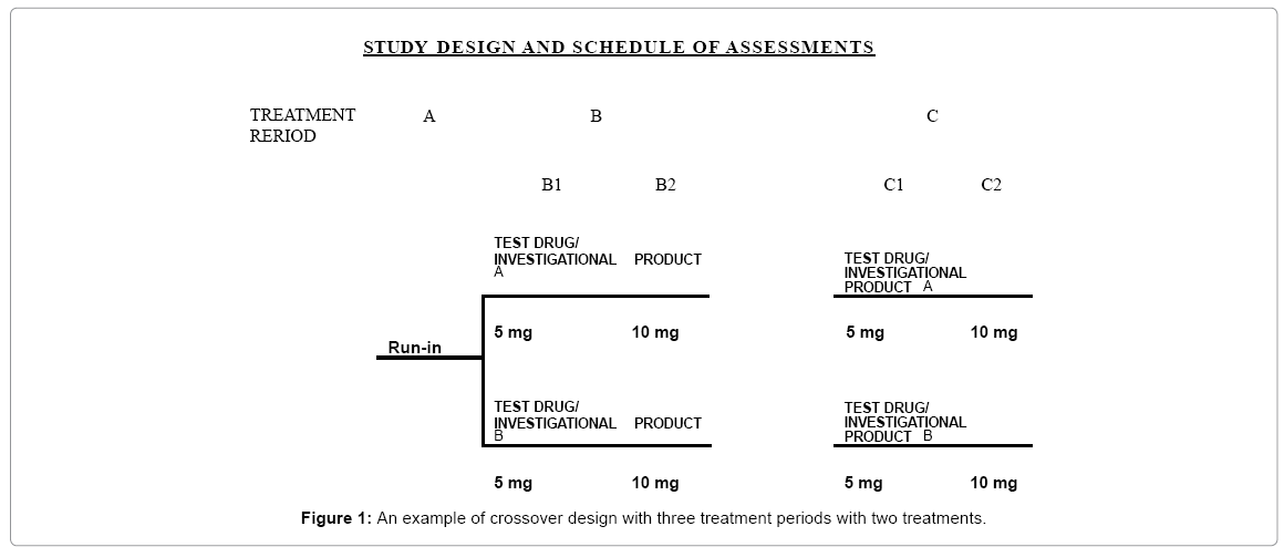
Figure 1: An example of crossover design with three treatment periods with two treatments.
For comparing more than two drug products, a Williams’ design is often considered. For example, for comparing three drug products, a six-sequence, three-period (6×3) Williams’ design is usually considered, while a 4×4 Williams’ design is employed for comparing 4 drug products. Williams’ design is a variance stabilizing design. More information regarding the construction and good design characteristics of Williams’ designs can be found in Chow and Liu [16].
Selecting an appropriate statistical design is critical in clinical development during the process of drug development. In recent years, there has been tremendous discussion on whether the choice of study design should be based solely on medical consideration. Another interesting question raised is whether to include marketing, regulatory, and/or statistical perspectives as well. Ideally an optimal design will account for considerations from different perspectives. In practice, however, such a design may not exist. It should be noted that considerations from different perspectives always mean limitations to the choice of design. Therefore, Temple [17] pointed out that a study must be sufficient to its task, and design limitations should be understood before proceeding, first to see whether a better design can be found and to understand the limits on interpretation imposed by a less than optimal design, and second, so that, it necessary, the limits can be discussed with the regulatory agency and potential problems are anticipated.
Parallel versus crossover
Crossover design: A crossover design is a modified randomized block design in which each block receives more than one treatment at different dosing periods. A block can be a patient or a group of patients. Patients in each block receive different sequences of treatments. A crossover design is called a complete crossover design if each sequence contains all treatments under investigation. For a crossover design it is not necessary that the number of treatments in each sequence be greater than or equal to the number of treatments to be compared. We will refer to a crossover design as a p×q crossover design if there are p sequences of treatments administered at q different dosing periods. Basically a crossover design has the following advantages: (1) it allows a within-patient comparison between treatments, since each patient serves as his or her own control. (2) It removes the inter-patient variability from the comparison between treatments. (3) With a proper randomization of patients to the treatment sequences, it provides the best unbiased estimates for the differences between treatments. The use of crossover designs for clinical trials has been much discussed in the literature Jones and Kenward [18], and Chow and Liu [16].
Parallel group design: A parallel group design is a complete randomized design in which each patient receives one and only one treatment in a random fashion. Basically there are two types of parallel group design for comparative clinical trials, namely, group comparison (or parallel-group) designs and matched pairs parallel designs. The simplest group comparison parallel group design is the two-group parallel design which compares two treatments (e.g., a treatment group vs. a control group). Each treatment group usually, but not necessarily, contains approximately the same number of patients. The ICH E9 [19] guideline “Statistical Principles for Clinical Trials” indicates that the parallel group design is the most common trial design for confirmatory trials (ICH E9, 1998).
Remarks: When planning a clinical trial, it is suggested that the relative merits and disadvantages of candidate statistical designs be compared before an appropriate design is chosen for the clinical trial. It is important to evaluate the suitability of the chosen design for addressing scientific/medical questions and/or claims. For example, if we are to choose between a crossover design and a parallel design for a clinical trial, we must first understand the nature of these two designs. For a parallel design, each patient receives one and only one treatment in random fashion, whereas for a crossover design each patient receives more than one treatment at different dosing periods. If a clinical trial is intending to investigate the residual effect that may be carried over from one treatment to another, a crossover design could be employed. Note that the Federal Register (Vol. 42, No. 5, Sec. 320.26(b) and 320.27(b), 1977) indicate that a bioequivalence trial (single dose or multiple dose) should be crossover in design, unless a parallel design or another design is more appropriate for some valid scientific reasons. On the other hand, if a clinical trial is intended to demonstrate the effectiveness and safety of a study medicine, a parallel design is more appropriate.
Cluster randomized design
The fundamental theory of the classic experimental design is based on the fact that the randomization unit is the same as the analysis unit used as the experimental unit for statistical inference. In clinical trials, the randomization units could be some social intact units such as family, school, worksites, athletic teams, hospitals, or communities. These social units are called clusters. The resultant randomized design with clusters as experimental units are referred to as cluster randomized design.
For cluster randomized designs, randomization is performed at the cluster level rather than at the subject level. Thus, the unit of analysis may not be necessarily the same as the unit of randomization. If the inference is made at cluster level, then the standard methodologies for traditional clinical trials provided can be applied because cluster is the unit of randomization as well as the unit of analysis. However, for most clinical trials with a cluster randomized design, the inferences are intended at the subject level, and hence, the standard methods for sample size calculation and data analysis considering subject as analysis unit are not appropriate. One of the major considerations for design and analysis of cluster randomized trials is the control of the intracluster and inter-cluster variations. As clusters are some intact social units such as families or worksites, therefore, we would anticipate that the subjects within the same cluster might share the same traits or have similar characteristics. In other words, the subjects within the same cluster are more similar than are those between clusters. One statistical measure to quantify this similarity is the intra-class correlation coefficient (ICC) If the intra-class correlation coefficient, denoted by ρ, is positive, the intra-cluster variation is smaller than the inter-cluster variation. The ICC plays a very important role in analysis of cluster randomized trials using subjects as the unit of inference.
Titration design
For phase I safety and tolerance studies, Rodda et al. [20] classify traditional designs as (i) rising single-dose design, (ii) rising singledose crossover design, (iii) alternative-panel rising single-dose design, (iv) alternative-panel rising single-dose crossover design, (v) parallelpanel rising multiple-dose design, and (iv) alternative-panel rising multiple-dose design Ting [21]; Chow and Liu [22].
Phase I studies are usually conducted in young, healthy male volunteers. The purpose of phase I studies is to obtain initial appraisement of drug safety through the evaluation of vital signs, physical health, and adverse events and frequent assessments of hematology, blood chemistry, and urine samples. The above designs are commonly employed in phase I safety and tolerance studies to efficiently provide the data that can be analyzed for generating hypotheses rather than for making definitive inference.
In medical practice, if the study medicine is intended for cancer or some life-threatening diseases, it may not be ethical to conduct phase I safety and tolerance studies on normal volunteers due to potential toxic or fatal effects. In addition results from animal studies provide little information regarding the therapeutic range for possible efficacy with tolerable safety. Due to the special characteristics of cancer patients and toxic profiles of cancer treatments, designs for cancer clinical trials require special considerations.
Adaptive design
In February 2010, the FDA [23] circulated a draft guidance on adaptive design clinical trials, which defines an adaptive design as a study that includes a prospectively planned opportunity for modification of one or more specified aspects of the study design and hypotheses based on analysis of (usually interim) data from subjects in the study. Analyses of the accumulating study data are performed at prospectively planned time points within the study, with or without formal statistical hypothesis testing. The FDA’s definition has been criticized for inflexibility in the sense that it is difficult, if not impossible, to consider all possible scenarios (to plan opportunities) ahead of time for clinical investigation of a test compound with complicated structure and certain uncertainties. The benefits and limitation of adaptive design are outlined in Table 13.
| Possible benefits | Limitations |
|---|---|
| Flexibility for identifying optimal clinical benefits in a more efficient way | Validity and quality/integrity are the major concerns due to possible optional bias caused by adaptions applied |
| Correct wrong assumption early | Statistical methods for some specific adaptive designs (e.g., less well-understood designs) are not well-established |
| Select the most promising option early | Criteria for decision-making may not scientifically justifiable |
| Make use of emerging external information | Statistical inference (e.g., p-value and CI) may not be reliable and the overall type I error rate may not be controlled |
| React to surprise (positive or negative) early | The role of Data Monitoring Committee (DMC) is not clear |
| Speed development process | There are some obstacles for implementation |
Table 13: Possible Benefits and Limitation for Utilizing Adaptive Designs in Clinical Trials.
As described in the 2010 draft guidance, the FDA classifies adaptive designs into two categories, namely “well understood” and “less well understood”. Well-understood designs are those that have been in use for years; the corresponding statistical methods are well established, and most importantly, the FDA is familiar with the study designs through the review of submissions utilizing them. In contrast, the relative merits and limitations of less well-understood designs have not yet been fully evaluated. Valid statistical methods have not yet been developed or established, and most importantly, the FDA does not have sufficient experience with submissions utilizing such study designs.
Depending upon the adaptations employed, adaptive designs can be classified into the following types: (i) an adaptive randomization design, (ii) an adaptive group sequential design, (iii) a flexible sample size re-estimation design, (iv) a drop-the-losers design, (v) an adaptive dose finding design, (vi) a biomarker-adaptive design, (vii) an adaptive treatment-switching design, (viii) an adaptivehypothesis design, (ix) a phase I/II or II/III adaptive seamless trial design, and (x) a multiple adaptive design Chow and Chang [24]. These designs are briefly described below.
Adaptive randomization design: An adaptive randomization design is a design that allows modification of randomization schedules based on varied and/or unequal probabilities of treatment assignment both prospectively and after the review of the response of previously assigned subjects. The purpose is to assign more subjects to promising test treatment under investigation and potentially to increase the probability of success of the intended trial. The commonly used adaptive randomization procedures include treatment-adaptive randomization, covariate-adaptive randomization, and responseadaptive randomization. In practice, an adaptive randomization design may be valuable in trials with a relatively small sample size or a trial with short-term outcomes, but may not be feasible for a large trial with relatively long treatment duration. Adaptive randomization is classified as a less well-understood design according to the FDA draft guidance (FDA, 2010) [23]. The issue regarding the balance of patient characteristics between the treatment groups is a concern for this type of design. The imbalance in important characteristics is problematic especially for confirmatory studies.
Adaptive group sequential design: An adaptive group sequential design is a classical group sequential design with pre-specified options of additional adaptations (e.g., sample size re-estimation, modification/ deletion/addition of treatment arms, change of study endpoints, modification of dose and/or treatment duration, and/or randomization schedules, etc.) at interim analyses. For the classical group sequential design, statistical methods and various stopping boundaries based on different boundary functions for controlling an overall type I error rate are available in the literature Chow and Chang [24]. Thus, the classical group sequential design is considered a well-understood design by the 2010 FDA draft guidance. However, with additional adaptations (e.g. sample size re-estimation based on unblinded interim analyses), the adaptive group sequential design may be a less well-understood design. In this case, standard methods for the classical group sequential design may not be appropriate, as it may not be able to control the overall type I error rate at the desired level of 5% due to potential issues pertaining to adaptations of a given study design. Appropriate statistical procedures are necessary to avoid the potential increase in the study-wide type I error rate (FDA, 2010).
Flexible sample size re-estimation design: A flexible sample size re-estimation design is referred to as a design that allows for sample size adjustment or re-estimation based on the observed data at interim. In general, sample size is determined before the trial formally starts based on pilot estimates of efficacy endpoints and their variability, or a best guess for the lowest clinically meaningful effect size between the treatment and control groups. Practically, parameter misspecification may be inevitable, which can lead to an underpowered design if the true variability is much larger than the initial specification of the variability (FDA, 2010). Thus, it is of interest to adjust sample sizes adaptively based on accrued data from the ongoing trial. However, sample size re-estimation suffers from the same disadvantage as the original power analysis for sample size calculation prior to the conduct of the study because it is performed by treating estimates of the study parameters, which are obtained based on data observed at interim, as true values. It should be noted that the observed difference at interim based on a small number of subjects may not be of statistically significance. In other words, the results observed from the study may be due to chance alone and cannot be reproducible. Thus, standard methods for sample size re-estimation based on the observed difference with a limited number of subjects may be biased and misleading (FDA, 2010). Sample size adjustment or re-estimation could be done in either a blinded Gould [25] which is based on overall data or unblinded fashion Cui et al. [26] which is based on the criteria of treatment effect-size, variability, conditional power, and/or reproducibility probability. In the FDA draft guidance, sample size re-estimation methods based on blinded interim analyses of aggregate/overall data are well-understood designs and they are recommended because these approaches do not introduce bias or impair interpretability. In contrast, statistical methods for sample size re-estimation based on knowledge of the unblinded treatmenteffect sizes at an interim stage of the study are considered less wellunderstood designs. Such designs may have the potential of increasing Type I error rate, which is the major regulatory concern for this class of designs. As indicated in the draft guidance, a statistical adjustment is necessary for the final study analysis to protect against such an increase of the type I error rate.
Drop-the-losers design: A drop-the-losers design is a design with multiple stages which allows (i) dropping the inferior treatment groups, (ii) modifying treatment arms, and/or (iii) adding additional arms after the review of accumulated data at interim. Drop-the-losers design is also known as selection design or pick-up-the-winner design. A drop-the-losers design is useful in phase II trials with the goal of finding the appropriate dose and frequency of dosing for later phase of clinical development. Typically, drop-the-losers design is the first stage of a two-stage design Thall et al. [27]. At the end of the first stage, the inferior arms will be dropped based on some pre-specified criteria. The winners will then proceed to the next stage. In practice, the study is often powered for achieving a desired power at the end of the second stage (or at the end of the study). In other words, there may not be any statistical power for the analysis at the end of the first stage for dropping the losers. In this case, effect size may be exaggerated and may consequently have a negative impact on future phase III study design. It, however, should be noted the investigator may be at risk of picking up the wrong dose group or dropping a group which contains valuable information regarding dose response of the treatment under study. Therefore, the selection criteria and decision rules play important roles for drop-the-losers designs. Figure 2 outline an example of using the adaptive model to drop the inferior treatment Chow and Change [24].
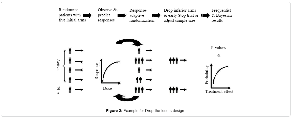
Figure 2: Example for Drop-the-losers design.
Adaptive dose finding design: An adaptive dose finding design is often used in early phase clinical development to identify the maximum tolerable dose (MTD), which is usually considered as the optimal dose for later phase of clinical development. In practice, it is undesirable to have too many subjects exposed to the dose limiting toxicity (DLT), while it is desirable to have a high probability for achieving the MTD with a limited number of subjects. Thus, the selection of initial dose, dose range, and criteria for dose escalation and/or dose de-escalation is important to the success of the adaptive dose finding design. The traditional “3+3” dose finding design is commonly used in the early phase of oncology studies. In recent years, several useful adaptive dose finding designs are proposed in the literature Pong [28]; a special issue of the Journal of Biopharmaceutical Statistics 17(6), 2007). Among those methods, continual re-assessment method (CRM) in conjunction with Bayesian approach introduced is usually considered Storer [29]. For the method of CRM, the dose-response relationship is continually reassessed based on accumulative data collected from the trial. The next patient who enters the trial is then assigned to the potential MTD level. However, a potential disadvantage is that the model may predict a higher MTD due to delayed response and/or a constraint on dose-jump O’Quigley et al. [30]. It is not uncommon that the sponsors propose CRM-based approaches in their regulatory submissions. In general, CRM-based approaches are considered to be more efficient than that of the commonly used “3+3” rule with respect to accuracy and the allocation of the MTD except when the true dose is among the lower levels. Note that drop-the-losers design and adaptive dose finding designs are best left to exploratory or early phase studies with the goal of obtaining information for designing subsequent studies.
Biomarker-adaptive design: A biomarker-adaptive design is a design that allows for adaptations based on the response of biomarkers. A biomarker is a characteristic that is objectively measured and evaluated as an indicator of normal biologic processes, pathogenic processes, or pharmacologic responses to a therapeutic intervention Iasonos et al. [31]. An adaptive biomarker design involves biomarker qualification and standard, optimal screening design, and model selection and validation. A biomarker-adaptive design is useful in the following ways: (i) identify patient population which is most likely to respond to the test treatment under study, (ii) identify natural course of disease, (iii) early detection of disease, and (iv) help in developing personalized medicine Freidlin and Korn [32]. It should be noted that correlation between biomarker and true clinical endpoint regardless of the treatment given makes a prognostic marker. A prognostic biomarker informs distinct expected clinical outcomes, which is independent of treatment. They provide information about the natural course of the disease in individuals who have or have not received the treatment under study. Prognostic markers may be used to separate good- and poor-prognosis patients at the time of diagnosis. In this case, stratification on prognostic biomarkers often improves design efficiency. However, prognostic markers cannot be used to guide to choosing a particular therapy Freidlin et al. [33]. On the other hand, correlation between biomarker and true clinical endpoint does not make a predictive biomarker. A predictive biomarker informs the treatment effect on the clinical endpoint, i.e. it identifies patients who are sensitive or non-sensitive to a given agent. Therefore, predictive markers can guide the choice of treatment methods. Biomarker-adaptive designs are typically used in exploratory studies which are important in selecting patient population for subsequent trials. However, as indicated in the draft guidance (FDA, 2010)), this type of design is considered less wellunderstood if it is imbedded in a confirmatory trial to modify patient eligibility criteria after the interim look. In such a situation, statistical adjustment is needed to avoid increasing the type I error rate Sargent et al. [34].
Adaptive treatment-switching design: An adaptive treatmentswitching design is a design that allows the investigator to switch a patient’s treatment from an initial assignment to an alternative treatment if there is evidence of lack of efficacy, disease progression, or safety of the initial treatment. Adaptive treatment-switching is commonly seen in oncology clinical trials due to ethical consideration Shao et al. [35]. In a cancer trial, estimation of survival (the clinical endpoint) is a challenge when treatment-switching has occurred in some patients. In practice, it is not uncommon that up to 80% of patients may switch from one treatment to another. Such a high percentage of subjects who switched due to disease progression could lead to change in hypotheses to be tested and cause further challenges in result interpretation Branson and Whitehead [36].
Adaptive-hypothesis design: An adaptive-hypotheses design is referred to as a design that allows modifications or changes in hypotheses based on interim analysis results. Modifications of hypotheses of ongoing clinical trials based on accrued data can certainly have an impact on the type I error rate, statistical power for testing the hypotheses with the pre-selected sample size for achieving the desired power. Some adaptive-hypotheses designs examples include pre-planned switch from a single hypothesis to a composite hypothesis or multiple hypotheses, pre-planned switch the null hypothesis and the alternative hypothesis, and pre-planned change due to switch between the primary study endpoint and the secondary endpoints.
Phase I/II (or Phase II/III) adaptive seamless design: An adaptive seamless design is a design that combines the study objectives, which are traditionally addressed in separate trials, into one single study. Most commonly used adaptive seamless designs include (i) adaptive seamless phase I/II design, and (ii) adaptive seamless phase II/III design. An adaptive seamless phase I/II design is referred to a design that combines a phase I trial which usually aims to find the maximum tolerated dose (MTD) for an investigational drug, and a phase II trial which examines the efficacy of the drug at the identified MTD. An adaptive seamless phase II/III design is a two-stage design consisting of a so-called learning or exploratory stage (phase II) and a confirmatory stage (phase III). An adaptive seamless design would use data from patients enrolled before and after the adaptation in the final analysis. Thus, an adaptive seamless design may reduce study sample size as compared to traditional designs. In addition, an adaptive seamless design is considered to be more efficient because there is no lead time between the two stages, i.e., the study moves to the second stage without holding the enrollment process. In practice, the sponsors often propose to use the so-called operationally adaptive seamless designs, in which two traditional trials (e.g. phase II and phase III) are conducted under a single study protocol but analyzed separately to address each objective using data from each stage. In this case, the investigators simply enjoy the saving in time. For an adaptive seamless phase II/III design, a typical approach is to power the study for the phase III confirmatory phase and obtain valuable information with certain assurance at the phase II learning stage. Its validity and efficiency, however, has been challenged. According to the draft guidance (FDA, 2010), an adaptive seamless phase II/III design is considered as a less well-understood design and may introduce bias. The type I error rate may be higher than stated in this design and could be a cause for concern.
Multiple adaptive design: A multiple adaptive design is a design with any combination of the above mentioned adaptive designs. A multiple adaptive design is more flexible but more problematic. Although a multiple adaptive design is more attractive, it makes good statistics practice (GSP) more difficult and challenging in practice.
Remarks: As noted in the draft guidance (FDA, 2010), the main concerns with designs that are less well-understood at this time include: (i) control of the study-wide Type I error rate, (ii) minimization of the impact of any adaptation associated statistical or operational bias on the estimates of treatment effects, and (iii) the interpretability of the results.
In this article, several commonly employed statistical designs in pharmaceutical/clinical development are reviewed. Following the concept of quality by design as recommended by the US FDA, these statistical designs are useful in non-clinical, pre-clinical, and clinical development of test compound under investigation to ensure that the test compound will possess good drug characteristics such as identity, strength (potency), quality, and purity (before approval) and safety, efficacy, quality, and stability (post-approval). Each design has its own merits and limitations under different circumstances at various stages of pharmaceutical/clinical development. As a result, how to select an appropriate design when planning a clinical trial is an important question. The answer to this question depends on many factors. As an example, for clinical development, these factors include (i) number of treatments to be compared, (ii) characteristics of the treatment, (iii) study objective(s), (iv) availability of experimental units (e.g., subjects or patients), (v) Inter-subject and intra-subject variabilities, (vi) duration of the study, and (vii) dropout rates.
In practice, as rule of thumb, Chow and Liu [22] suggested that for a multicenter trial, the number of centers (study sites) should not be greater than the number of subjects in each center for achieving optimal statistical properties.