Arsenic (As) occurs naturally in rocks and water. Sources of arsenic in groundwater include the weathering of sulfide minerals, desorption from sediments under alkaline conditions, evaporation processes in closed and arid basins, volcanic rocks, and geothermal waters [1]. Consuming high concentrations of arsenic in drinking water can create health problems including bladder, lung, and skin cancers [2]. The U.S. Environmental Protection Agency Maximum Contaminant Level (MCL) for total arsenic in drinking water was reduced from 50 to 10 micrograms per liter (μg/L) in January 2001, and compliance with this standard was required beginning in January 2006.

Arsenic naturally sorbs onto oxide surfaces of mineral grains in sedimentary material. Two primary triggers are associated with arsenic mobilization into groundwater: (1) High pH values, particularly above pH 8.5, which can release arsenic sorbed to iron, manganese, and aluminum oxides on the surfaces of mineral grains under oxic conditions, and (2) Anoxic conditions, which can induce reductive dissolution of iron and manganese oxide coatings on mineral grains, releasing sorbed arsenic [3,4].

High concentrations of arsenic in groundwater have been identified in many areas of the USA, including Alaska, New England, some of the interior plains states, and the southwestern states of Nevada, California, and Arizona [3]. Arid regions of the southwestern United States often depend on groundwater resources to supply rapidly growing populations. Arsenic is in water from some wells in the Mojave River basin in the western Mojave Desert of southern California at concentrations in excess of the MCL for arsenic [5-8].

This study well is in the Mojave River basin and Mojave Desert near Victorville, California, about 97 km northeast of Los Angeles (Figure 1). The population of Victorville has increased from 64,029 in 2000 to 120,336 in 2008. The demand for groundwater has increased with population growth, and withdrawals exceed natural recharge. Pumping in excess of recharge since the mid-1940s has resulted in a decline in groundwater levels, degradation of groundwater quality, and land subsidence [9,10]. Arsenic concentrations from the Ground Water Ambient Assessment (GAMA) Program sampling, combined with California Department of Public Health (CDPH) sampling, in the Mojave River basin 2000 to 2008) ranged from less than 2 μg/L to more than 50 μg/L and 21 wells had arsenic levels in excess of the USEPA MCL for arsenic of 10 μg/L. Well 5N/4W-31A1S near Victorville has a history of arsenic concentrations exceeding the MCL. In February 2008, the arsenic concentration in the surface discharge from this well was 17 μg/L.

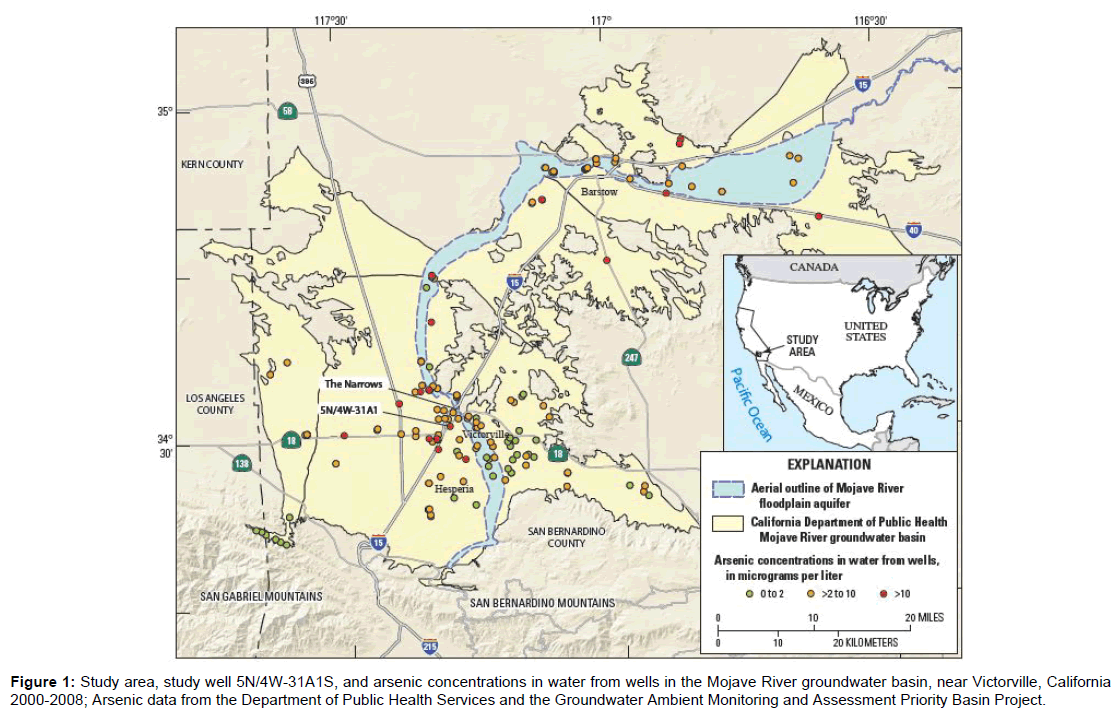
Figure 1: Study area, study well 5N/4W-31A1S, and arsenic concentrations in water from wells in the Mojave River groundwater basin, near Victorville, California 2000-2008; Arsenic data from the Department of Public Health Services and the Groundwater Ambient Monitoring and Assessment Priority Basin Project.

Treatment strategies for water having high-arsenic concentrations include arsenic removal through coagulation/filtration and iron oxide adsorption [11,12]. Low-arsenic waters can also be blended with higharsenic water from different sources to meet water quality standards. However facilities for arsenic mitigation using these methods are costly to construct and operate.

Another approach applicable in some groundwater settings is well modification [4,13]. The well-modification approach identifies zones of poor water-quality encountered by the well using coupled wellbore flow and depth-dependent water-quality data. This information is used to identify intervals having poor-quality water and modify the well construction to seal off those intervals from the well, thereby preventing poor quality water from entering the well and improving the quality of water yielded by the well. This method has been shown to inexpensively reduce high concentrations of contaminants such as chloride and arsenic in water from wells [14-16].

A study of high-arsenic concentrations in water from wells in the San Joaquin Valley near Stockton, CA by Izbicki et al. [4] demonstrated that well modifications in unconfined alluvial deposits could reduce arsenic concentrations in the surface discharge from wells to below the MCL. In comparison with the Mojave Desert, the alluvial deposits of the Stockton area are relatively more fine-textured and the wells were completed at shallower depths. Halford et al. [17] showed that well modification could reduce arsenic concentrations from more than 50 μg/L to 3 μg/L in water from a well in Antelope Valley, within the Mojave Desert about 80 km northwest of Victorville, CA. However, in the Antelope Valley, deeper high-arsenic water was separated from shallower low arsenic water by a thick, low-permeability lacustrine clay deposit that limited the upward movement of high-arsenic water to the modified well. This study examines a well drilled into unconfined alluvial deposits of the Mojave Desert that has high-arsenic water.

The Upper Mojave River Groundwater Basin has an arid climate, characterized by low humidity, low precipitation, and high summer temperatures [18,19]. Surface drainage is through the Mojave River, which originates in the San Bernardino Mountains, and flows north through Victorville [18]. The Mojave River flows only intermittently after winter storms; during the summer months, the river is dry [20]. Because of the lack of perennial streamflow, groundwater is the only dependable source of water supply in the area and is the focus of this study.

The Mojave River Groundwater Basin contains an unconsolidated alluvial aquifer along the Mojave River called the floodplain aquifer, Holocene to Pleistocene in age, consisting of sand and gravel weathered from granitic rocks in the San Gabriel and the San Bernardino Mountains [21]. The floodplain aquifer is typically less than 80 meters thick, surrounded and underlain by the more areally extensive regional aquifer, composed of basin fill and alluvial fan material deposits, Holocene to Miocene in age, eroded from the San Bernardino and the San Gabriel Mountains [9,22]. Consolidation of the regional aquifer deposits increases with depth [23]. Near Victorville, surrounding and underlying the floodplain aquifer, the regional aquifer includes deposits from the ancestral Mojave River. The ancestral Mojave River deposits are Pleistocene to Pliocene in age and range in depth from about 130 m to almost 200 m in thickness [9]. The ancestral Mojave River deposits are highly-permeable compared to the alluvial fan and basin fill material elsewhere in the regional aquifer. The regional aquifer contains a large amount of groundwater in storage; however, recharge is small in comparison with the floodplain aquifer [9]. As a consequence, some water in the regional aquifer was recharged more than 20,000 years ago [20,24,25]. This water has reacted extensively with minerals in aquifer deposits and is often highly alkaline with pH exceeding 8.0 in deeper deposits [24]. Many trace elements, such as arsenic, are soluble in groundwater under these conditions.

Well 5N/4W-31A1S was drilled in 2003 and screened within the regional aquifer, although most of the perforated interval is within ancestral Mojave River deposits. The well is 213 m deep and is screened from 151 to 154 m, 159 to 163 m, 166 to 171 m, 175 to 180 m, 189 to 201 m, and 209 to 213 m bls (Figure 2). The perforations from 151 to 201 m bls are within the ancestral Mojave River deposits. The deeper perforations are within the underlying alluvial fan and basin-fill deposits. During May 2008, the static water level was approximately 104 m bls. When pumped, the well yield was 190 L/s, and the pumping water level was approximately 130 m bls (26 m of drawdown).

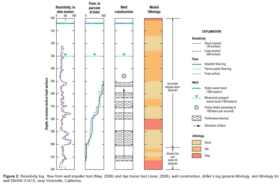
Figure 2: Resistivity log, flow from well impeller tool (May, 2008) and dye tracer tool (June, 2008), well construction, driller’s log general lithology, and lithology for well 5N/4W-31A1S, near Victorville, California.

Purpose and scope

The purpose of this study was to evaluate the well modification method as an alternative approach to arsenic mitigation in a publicsupply well in relatively deep unconfined alluvial deposits of the Mojave Desert. Well 5N/4W-31A1S, operated by the city of Victorville, was selected for this study because it contained arsenic concentrations in excess of the MCL of 10 μg/L. The scope of the study included collecting well-bore flow and depth-dependent water-quality. The data were related to aquifer property and hydraulic data, and interpreted using the computer program AnalyzeHOLE [13]. This study was completed as part of the USGS-GAMA Ambient Priority Basin Project in California.

Coupled well-bore flow and depth-dependent water samples were collected from well 5N/4W-31A1S in May and June of 2008. Well-bore flow was measured under pumping conditions using a commercially available impeller flowmeter and using the tracer-pulse method [26,27]. Water levels were measured in the well and the pumping rates were recorded throughout the logging of the well. Pumping and drawdown data collected over a 4-hour period were used to calculate aquifer transmissivity using the Cooper-Jacob method, a simplification of the Theis solution for unconfined aquifers [28]. Water at specific depth intervals within the well, selected on the basis of the well construction and velocity log data, was sampled under pumping conditions using a gas-displacement pump with a diameter of less than 2.5 cm [27].

The impeller -flow logs were collected by trolling the tool downward though the well at three rates: approximately 10, 20, and 30 m per minute (actual trolling rates were 9, 18, 27 m per minute). Access to the well was through a specially designed tube (commonly known as a camera tube) that entered the well below the pump intake.

Well-bore flow logs were examined for consistency. Data from the three trolling rates were used to calibrate the impeller tool and to evaluate the precision and sensitivity of the tool (Appendix A).

The dye tracer-pulse method measures flow and uses a high pressure hose equipped with valves to inject rhodamine dye at known depths in a well [20,27]. The arrival of the dye at the surface discharge of the well is measured. For an interval within the well, a flow velocity is calculated from the difference in arrival times between the two injection depths that bracket the interval. A velocity profile was constructed from a series of such injections at different depths in the well (Figure 2). The dye tracer-pulse flow log measurements were collected at 11 depths above screened intervals and within screened intervals to determine the velocity profile within the well. For this study, dye tracer-pulse logs were analyzed using the first arrival and the peak arrival times (Figure 2). The first arrival time is when the injected rhodamine dye was first measured in the well water at surface distribution. The peak arrival is when the maximum amount of rhodamine dye was measured in in the well water at the surface distribution.

The impeller-flow logs were compared with the dye tracer-pulse flow logs to confirm estimates of flow into the well. It was useful to use both methods to identify intervals of low flow and high-yield flow into the well. Although results from both logs are similar, the impeller logs can define flow into the well with greater resolution than the tracerpulse logs for aquifers where thin intervals contribute large amounts of flow into the well therefore the final interpreted log used for model simulations was derived from the impeller-flow log. The key depth dependent water-quality parameters pH and dissolved oxygen were

measured. These parameters were chosen as it is high pH values and very low dissolved oxygen that trigger desorption of arsenic from aquifer material. Groundwater samples collected to be analyzed for major and minor ions and trace elements, including arsenic, were filtered and preserved in the field and shipped within 24 hours to the USGS National Water Quality Laboratory (NWQL) in Denver, CO (Appendix A). The water-quality profile for arsenic was constructed from sample results from 7 depths including at land surface (Figure 3). The concentrations of arsenic (Ca) at the first sample depth (C₁) and the next sample depth (C₂) were used with velocity-log flow data at the first sample depth (Q₁) and the next sample depth (Q₂) to calculate the arsenic concentration in the water entering the well from the adjacent aquifer zone [27]:

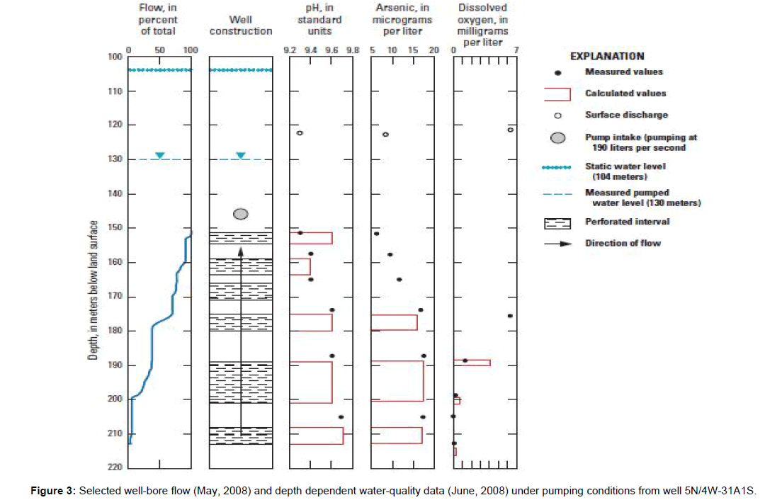
Figure 3: Selected well-bore flow (May, 2008) and depth dependent water-quality data (June, 2008) under pumping conditions from well 5N/4W-31A1S.

Equation 1: (Ca) = [(C₁Q₁-C₂Q₂)/Qa]; where Qa = (Q₁ - Q₂)

Well-bore flow data

The impeller -flow log and dye tracer-pulse result profiles show two high-yield water-bearing zones within the well (Figure 2). Both first arrival and peak arrival dye tracer-pulse logs are plotted (Figure 2), the methods produced similar results. The first high-yield zone corresponds with the screen from 175-180 m bls and produces approximately 30 percent of flow; the second zone corresponds with the screen from 189- 201 m and also produces approximately 30 percent of flow into the well. Both these zones are within the ancestral Mojave River. The upper three screened intervals within the well contribute only small amounts of flow (Figure 2). Two of the intervals correspond to relatively low resistivity values on the resistivity log collected at the time the well was drilled. However, the uppermost interval is within a more resistive unit that may have been expected to yield more water to the well. Geologic and geophysical data collected from a well at the time of drilling are indirect measures of potential well performance, well-bore flow data are a more direct measure of well performance that integrates the hydraulic properties of the deposits encountered by the well and how these deposits are connected to deposits farther away from the well when the well is pumped. Within the basin-fill deposits, flow into the screen from 209-213 m bls was only 8 percent of the total yield (Figure 2).

Water-chemistry data

Depth-dependent samples collected within the well under pumping conditions show that pH and arsenic concentrations increase with depth while dissolved oxygen concentrations decrease with depth (Figure 3). Arsenic concentrations in samples from the well ranged from 6.4 to 17.6 μg/L. High concentrations of arsenic, greater than the MCL of 10 μg/L, enter the well from the aquifer below 166 m bls. Most of the arsenic enters the well from the screened intervals between 189 and 213 m bls where approximately 38% of the total inflow enters the well.

Arsenic concentrations begin to increase in the well at a depth of 166 m within the high-water yielding ancestral Mojave River deposits and above the low-yielding underlying alluvial fan and basin fill deposits. Dissolved oxygen concentrations begin to decrease at this depth (Figure 3) and arsenic concentrations in this area may be controlled by geochemical factors, such as pH and redox at deeper depths, rather than geologic factors, such as the source of the alluvial deposits. Increasing arsenic concentrations with depth agrees with water-quality data for arsenic concentrations reported in Mojave River basin monitoring wells [6].

Simulation of well-bore flow

The computer program AnalyzeHOLE, a well-bore analysis tool, was used to simulate groundwater well-bore flow and arsenic concentrations in well 5N/4W-31A1S and the adjacent aquifer [13]. The program uses MODFLOW to simulate axially-symmetric, twodimensional radial flow to the well in response to pumping. MODPATH a particle-tracking program embedded within AnalyzeHOLE, was used to calculate arsenic contributions before and after simulated well modifications [29,30].

The simulation consists of a cylinder of aquifer material with a radius of 6.1 × 10⁴ m and a thickness of 143 m; the simulation grid has 76 variably-sized columns in the lateral direction and 100 rows of uniform thickness in the vertical dimension (Figure 4). This large simulated volume was used to ensure that lateral no-flow boundaries are beyond the pumping effects of the well. Hydrologic conductivities were initially assigned to the simulation on the basis of aquifer lithology described in the driller’s log [31]. Aquifer transmissivity was estimated to be 1,200 m²/day using measured drawdown and well during sampling. The observed pumping rate of 190 L/s during sampling was the pumping rate used in the simulations.

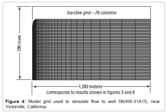
Figure 4: Model grid used to simulate flow to well 5N/4W-31A1S, near Victorville, California.

The computer program MODPATH was used to simulate the movement of water particles within the simulation. For numerical purposes, particle movement was simulated as injection rather than withdrawal and the simulation assumes withdrawal is the mirror image of the injection [30]. To simulate pumping using this approach, the pumping water level within the simulation was approximated using the Theis equation and did not change during the simulation. The error induced by this approximation is believed to be small [17]. Movement of water to the well is shown as the particle pathlines that track particle movement in response to simulated pressure changes in the well from simulated pumping. Each cell of the simulation grid contained one particle that represents a discrete fraction of water contribution to the well with a unique water quality. The water quality produced by well 5N/4W-31A1S was calculated as the flow-weighted average of the particle concentrations. Arsenic concentrations for particles within the model ranged from 2 to18 μg/L.

The simulation was calibrated by adjusting the hydraulic conductivity of simulated aquifer material within reasonable ranges, from less than 1 to 15 m/day, to match the measured impeller-flow log data and observed drawdown while maintaining a constant transmissivity (Figure 5). The hydraulic conductivity of clay, silt, and sand are paired with lithology in Figure 5. The measured water-level decline (26 m) during pumping was simulated within 1 m using the estimated transmissivity value 1,200 m²/day and assigned hydraulic conductivities.

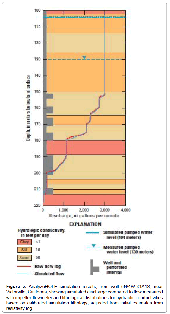
Figure 5: AnalyzeHOLE simulation results, from well 5N/4W-31A1S, near Victorville, California, showing simulated discharge compared to flow measured with impeller-flowmeter and lithological distributions for hydraulic conductivities based on calibrated simulation lithology, adjusted from initial estimates from resistivity log.

Simulations were generated to evaluate how well yield and arsenic concentrations in the surface discharge of the well would vary in response to changes in well construction. The first simulation used the existing well construction (213 m depth) to generate drawdown and particle movement; in each additional simulation, screened intervals were eliminated one at a time and the simulation was run to evaluate the arsenic concentrations to changes in the well construction. The time period for each simulation was 1,000 days of pumping.

The simulated drawdowns and particle movement generated for well 5N/4W-31A1S during a 1000 day period are shown in Figure 6. The simulated drawdown of 27 m compared closely to the measured drawdown of 26 m during well sampling. The simulated particles of water moved faster through more permeable deposits, and particles near the water table moved steeply downward until encountering coarse-grained aquifer material where upon they moved toward the well Figure 6. The simulated arsenic concentration in well surface discharge water was 8.8 μg/L which compares closely to the sampled arsenic concentration of 8.4 μg/L.

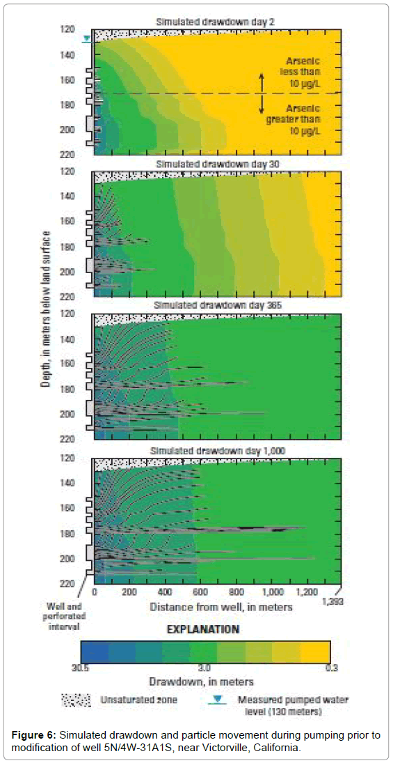
Figure 6: Simulated drawdown and particle movement during pumping prior to modification of well 5N/4W-31A1S, near Victorville, California.

Simulated drawdown and particle movement during pumping, after the two deepest screened intervals were removed from the simulated well are shown in Figure 7. High-arsenic water that had entered through the two deeper screened intervals no longer entered the well directly, but some of this water did move up through aquifer material and enter through the deepest remaining screen interval. Arsenic concentrations in surface discharge in the simulation of the modified well decreased to 6.7 μg/L and remained constant for the remainder of the 1,000 day simulation. This value represents about a 25% decrease in arsenic concentration. Elimination of the two deepest screened intervals resulted in a simulated decrease in well yield of 30 percent.

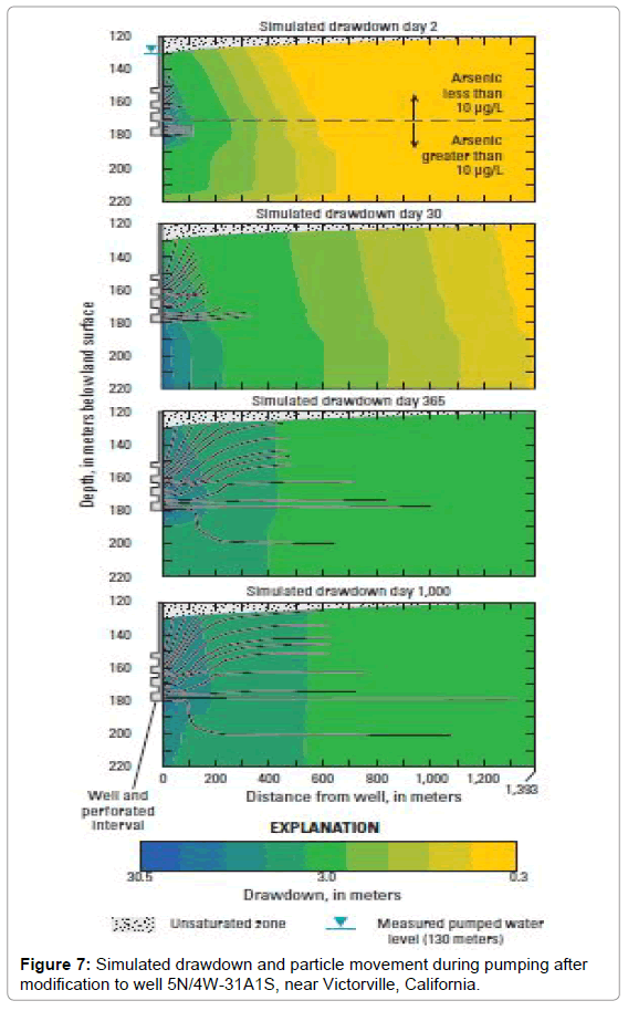
Figure 7: Simulated drawdown and particle movement during pumping after modification to well 5N/4W-31A1S, near Victorville, California.

Additional simulations were run to calculate the change in arsenic concentrations in surface discharge after one, then two, then three of the lower three screened intervals were eliminated (Figure 8: scenarios 2-4). There was little change in arsenic concentration after removing the deepest screen interval, which is consistent with the low yield measured at that depth. Decreases in simulated arsenic concentrations in the surface discharge of the well were approximately 2 μg/L in scenario 3 when the second deepest screened interval was removed. The lowest arsenic concentrations were in scenario 4, in which the third deepest screened interval was sealed. However this simulation also resulted in the greatest yield reduction of 70%. The simulated arsenic concentrations in all tested scenarios were initially low then increased during the first 100 days of simulated pumping to a steady-state concentration for the remainder of the 1,000 day simulation as deeper water moved upward through the aquifer in response to pumping.

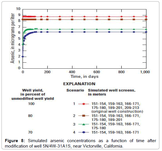
Figure 8: Simulated arsenic concentrations as a function of time after modification of well 5N/4W-31A1S, near Victorville, California.

The simulation sensitivity to changes in porosity, vertical anisotropy, specific storage, and specific yield was tested. Porosity, vertical anisotropy, specific storage, and specific yield were increased and/or decreased then the simulation was run to observe results. Changes in these input parameters had little to no effect on simulation results. The simulation sensitivity to bore-hole flow and drawdown was tested. The simulated bore-hole flow and drawdown were most sensitive to the changes in hydraulic conductivity. When lithological units with the conductivity values of sand were increased or decreased it produced deviations from the measured flow log and transmissivity.

The simulation developed to interpret well-bore flow and depthdependent water-quality data from well 5N/4W-31A1S is a simplified two-dimensional radial representation of the surrounding regional aquifer flow system. The simulation assumes aquifer materials are flat-lying and areally extensive and does not account for no-flow boundaries, regional changes in subsurface geology, hydraulic variations, or interactions between surrounding pumping wells. The flow simulation is intended to be a simple tool useful for evaluating the effects of well design modifications on surface discharge water-quality and not an accurate representation of the regional groundwater flow field near the well.

Coupled well-bore flow and depth-dependent water-chemistry data show that arsenic concentrations and pH values increase with depth in well 5N/4W-31A1S while dissolved oxygen concentrations decrease with depth. Increases in arsenic concentrations in reducing conditions (dissolved oxygen less than 0.5 μg/L) below 175 m are consistent with reductive dissolution of iron hydroxide coatings on mineral grains and subsequent mobilization of arsenic. Arsenic concentrations change abruptly at the 175 m depth, increasing from less than the detection limit of 10 μg/L to almost 17 μg/L. This increase is controlled by changing redox conditions and does not occur at the geologic contact between the ancestral Mojave River deposits and the underlying basin-fill and alluvial fan deposits. Ancestral Mojave River deposits contribute most of the water to this well.

Data interpreted using AnalyzeHOLE to evaluate the effects of changes in the simulated well design on arsenic concentrations confirms that sealing off the bottom two screened intervals reduced simulated arsenic concentrations entering the well by about 25 percent to 6.7 μg/L and reduced the in well yield by 30 percent.

Water purveyors in the Mojave River groundwater basin near Victorville could benefit from modifying existing wells to reduce arsenic concentrations and from carefully designing future wells to ensure they do not penetrate depths containing high-arsenic groundwater. Results of this study show that this well yielding water exceeding arsenic concentrations above the MCL could be simply and cheaply modified to reduce arsenic concentrations to meet drinking water standards. Also high arsenic water could be avoided by drilling future wells to depths equal or lesser than 180 m bls. Such sampling methods, simulations, and well modification could also be used to target and address high concentrations of other trace elements such as chromium, in public supply wells.

The authors thank the GAMA Priority Basin Project for funding, and the Victor Valley Water District for well access and water-quality data. The authors also thank Christina Stamos, Nick Teague, Keith Halford, Joseph Montrella, and Gregory Smith of the USGS for assistance with collecting and data interpretation.

Well-bore flow was measured under pumping condition using an impeller flowmeter in well 5N/4W-31A1S to provide well yield. To develop a calibration for well-bore flow, intercepts of the lines, 9 meters/minute and 18 meters/minute, were plotted against the difference in the trolling rates, 18 and 27 m/minute. This comparison of linear regression lines had a slope of approximately 1. This result indicates that the tool output was linear over the range of measured flow and suitable to develop a field calibration for the meter. The well-bore flow data was plotted with depth and adjusted by assuming zero flow into the well in blank (unscreened) casing intervals (Figure 2).

Water-quality samples were collected with a small diameter (less than 2.5 cm) gas-displacement pump. Water-quality samples collected at each well depth are a mixture of water from all the screened aquifer zones below the depth at which the sample was collected [14,27]. Samples were collected in accordance with the protocols established by the USGS National Water Quality Assessment (NAWQA) program and the USGS National Field Manual [32]. Arsenic was analyzed at the USGS NWQL by inductively coupled plasma mass spectrometry (ICP-MS) [33].