Journal of Geology & Geophysics
Open Access
ISSN: 2381-8719
ISSN: 2381-8719
Research Article - (2021)Volume 10, Issue 8
Sediment bed shear stress is well known to effectively contribute to the entrainment of sediment grains from parent bed as well as in the initiation of grain motion into suspension flow. Direct measurement of the magnitude of bed shear stress in varying field conditions has always presented difficult challenges hence it is estimated from observations and analysis of flow velocity fluctuations above the flow bed.
Reports of some recent researches have shown poorer agreement in estimates of bed shear stresses from existing multiple sources including the bed slope, log profile, Reynolds stress distribution, turbulent kinetic energy and this raises questions with regards to the estimates validity. Estimates obtained for bed shear stresses from multiple methods are expected to show considerable agreement using similar sets of flow data.
This paper reports the investigation carried out to determine the consistency and possible correlation in bed shear stress estimates or otherwise obtained from multiple estimation methods, using an unusually large flow fluctuating velocity dataset obtained from a laboratory flume tank experiment instrumented with a three-component (3-C) Acoustic Doppler Velocimeter (ADV).
The analysis of results and comparison of estimates from three methods suggest a significant consistency in estimates especially estimates using the log profile and Reynolds stress methods. However, estimates from the bed slope methods seemed to be relatively higher with up to 26% as in experimental case 5, when compared to the other two methods. These research findings further affirm the reliability of existing methods of bed shear stress evaluation especially the log profile and Reynolds stress.
Bed shear stress; Flow velocity; Reynolds shear; Log profile
Despite over a century of sustained research into how sediment grains are entrained from the parent bed and transported in open channels, the need to improve understanding of the actual mechanism, has continued to prompt active research in this multifaceted sub-field of sedimentology.
Bed shear stress, τ 0 is a major parameter that facilitate the dislodgement of sediment grains from the bed as well as define the initiation of grains motion into flow and cause resistance to the overlying flows [1-4]. Bed shear stress is a fundamental variable in fluvial process and a very significant parameter required in estimating sediment transport rates, predicting transport of environmental contaminants and the prediction of resistance coefficients in open channels, streams, and rivers [5].
For a moving turbulent flow, bed shear stress is a direct function of the flow depth h, the bed slope s and indirectly a function of the flow velocity. It is proportional to the square of the flow velocity. Over the years, direct measurements of bed shear stress in relation to sediment grains transport have been practically impossible both in the field and controlled laboratory environment. However, owing to the practicality of measurement and application, bed shear stress is most commonly represented by a mean value, averaged over the width of the channel, so that:
Where ρ is fluid density, g is the gravitational acceleration, h is the flow depth and s is the mean longitudinal water surface slope.
Bed shear stress is also inferred from the analysis of the measured flow velocity fluctuations. There is a direct relationship between bed shear stress, τ0 and the flow shear velocity, u* as expressed in equation 2, below [6].
Where 0 τ is the bed shear stress, u* is the shear velocity, and ρ is the fluid density.
Due to the challenges of direct measurements, numerous methods are used to estimate bed shear stress such as the bed slope method, log profile (from the gradient of a logarithmic profile) and Reynold’s stress decomposition method.
The key issue this paper seeks to address is the consistency and possible correlation of bed shear stress estimates obtained from multiple estimation methods. Estimates obtained for bed shear stresses from several methods are expected to show considerable agreement using similar sets of flow data. However, published reports from recent researches show poorer agreement in bed shear stress estimates which raises questions with regards to the validity of estimates. For example, obtained significantly different bed shear stress estimates from four different approaches in their study of the variation of bed shear stress with downstream distance with changes in bed roughness [7]. Also in Lee ZS and Baas AC research, they observed discrepancies in bed shear measurement estimates from three main sources such as the Log profile, Slope and Reynolds decomposition methods [1]. Nezu and Nakagawa had estimated ± 30% variability range for bed shear stress values when comparing estimates from the logarithmic profile and the Reynolds stress methods with the slope method and also hinted that the variability increases with bed roughness [8]. Biron et al. have also compared results from multiple bed shear stress estimates in laboratory experimental flows over sand, plexiglass and artificial deflectors and observed that the logarithmic profile methods gave bed shear stress estimates that were significantly higher than the Reynold’s as well as other methods [9]. In contrast, field experiments obtained comparable estimates using direct Covariance (COV) measurement, Turbulent Kinetic Energy (TKE), inertial dissipation and velocity-profile methods [10].
Methods of bed shear stress estimation
Several approaches were suggested by Nezu and Nakagawa for the estimation of bed shear stress, however, this paper focusses on three different approaches namely, the bed slope, log profile and the Reynolds stress distribution [8].
Bed slope method (under conditions of uniform flow)
This is one of the most common methods of evaluating bed shear stress and it is most effective under conditions of uniform flow. The bed shear stress is calculated from the bed slope value s and flow section characteristics [6,11]. The bed shear stress is defined by the relation as in equation (1), however, according to Biron, this method may not be appropriate for local, small-scale estimates of the variation in shear stress [9].
The Log Profile (LP) method
This method mainly relies on near-bed, time-averaged local flow velocity measurements taken at several elevations within the log layer (at least two, commonly three or four, preferably more) [12]. The primary practical consideration of the log profile method is the need to measure flow velocities at several points, possibly with intrusive (flow-disturbing) sensors. The logarithmic velocity profile is expressed by the von Karman-Prandtl equation. The equation expresses the logarithmic relation between the shear velocity and the variation of mean velocity with height [9,13,14].
It is given by
Where u* is the shear velocity, u is the time-averaged flow velocity at elevation z above the bed, z0 is the roughness height,κ is the von Karman’s constant.
The log profile method is particularly valid only for steady flows [15].
The bed shear stress is calculated as a function of u* , which is determined by fitting a linear relation between ln (z) and u(z) and extracting the slope to the fit to yield [16,17]:
The log profile method is appropriate for estimating bed shear stress in both the field and open channel flows [8]. However, the limitations of using this method for reliable estimates are where the underflows have gravel beds [18]. Lamb also observed that this method may not be very suitable for flows with grain sizes of same order as the depth [19]. Similarly, Etminan noted that the method is unreliable for flows with relatively large roughness heights with elements such as ripples, gravels and vegetation [20].
The Reynolds stress decomposition method
It is based on the distribution of Reynolds stress. In a fully turbulent flow, where there are measurements of turbulence, the shear stress is estimated from the relation (Table 1).
| Method | General principles | Equation |
|---|---|---|
| Slope method | Relies on the force balance equation |  |
| Log profile | Fitting of the experimental velocity profile to the turbulence model. | 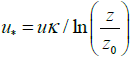 |
| Reynolds stress | Direct measurements of velocity fluctuations of the streamwise and vertical components | 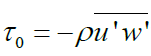 |
Table 1: Outline of some of the methods of bed shear stress estimation.
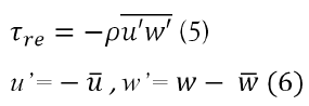
where ρ is the flow density, u’ is the turbulent fluctuation velocity in the direction of flow and w’ is the turbulent velocity fluctuation in the vertical direction [21,22].
The Reynolds stress method may not be appropriate for field studies due to errors arising from any tilting of the sensor or from secondary flows [10].
Datasets and methods
Data for this research was generated from flow experiments carried in the Sorby Fluid Dynamics Laboratory at the University of Leeds, United Kingdom. The laboratory facility comprises of an 8.5 m long, 0.34 m deep and 0.3 m wide tilting, rectangular and recirculating glass-sided flume instrumented with a Three- Component (3-C) Acoustic Doppler Velocimeter (ADV).
The measuring system which comprised mainly the Acoustic Doppler Velocimeter was positioned at the centre of the flume, about 4.2 m from the downstream end of the flume (Figure 1) and all flow velocity measurements were taken at the centreline of the cross section. Six flow experimental cases were designed for this investigation with unique conditions such as varying discharge rate, flow height/thickness, type of bed floor (roughness) as well as the slope of the flume (Table 2). The details of the methods of data collection and processing have been fully described [23].
| Flow cases | Bed lithology | Bed slope | Density (kg/m3) | Discharge rate Q/m3/h |
Mean velocity (m/s) |
|---|---|---|---|---|---|
| Case 1 | very fine sand | 0.0007 | 1000 | 0.022 | 0.36 |
| Case 2 | fine sand | 0.0011 | 1000 | 0.04 | 0.551 |
| Case 3 | Gravel | 0.0012 | 1000 | 0.025 | 0.333 |
| Case 4 | Gravel | 0.0016 | 1000 | 0.031 | 0.512 |
| Case 5 | Gravel | 0.0018 | 1000 | 0.022 | 0.443 |
| Case 6 | Gravel | 0.002 | 1000 | 0.033 | 0.616 |
Table 2: Summary of flume hydraulic data and flow conditions for all six experimental cases.

Figure 1: The signal receiving beams of an ADV used for flow velocity data collection.
Data analysis
The results of bed shear stresses obtained from three different approaches such as bed slope, log profile and Reynolds stress is presented below.
Bed slope method
With an assumed gravitational acceleration of 9.81, equation 1 was used to estimate the bed shear stress needed to entrain sediment grains into suspension flow. The bed shear stress estimates averagely ranged between 0.3430 to 2.9400 Nm-2 for all six experimental flow cases and are presented in Table 3 below. The bed shear stress estimates using this method is applicable mostly to steady uniform flow. An important observation is that the shear stresses increase with increase in grain size, flow height as well as bed slope.
| Flow cases | Nature of flow bed | Sensor height (m) | Bed slope | g (m/s) | Density (kg/m3) | Bed shear stress (Nm-2) | Uncertainty |
|---|---|---|---|---|---|---|---|
| Case 1 | fine sand | 0.05 | 0.0007 | 9.8 | 1000 | 0.3430 | ± 0.00012 |
| Case 2 | fine sand | 0.08 | 0.0011 | 9.8 | 1000 | 0.8624 | ± 0.000126 |
| Case 3 | Gravel | 0.09 | 0.0012 | 9.8 | 1000 | 1.0584 | ± 0.000146 |
| Case 4 | Gravel | 0.1 | 0.0016 | 9.8 | 1000 | 1.5680 | ± 0.00016 |
| Case 5 | Gravel | 0.12 | 0.0018 | 9.8 | 1000 | 2.1168 | ± 0.00015 |
| Case 6 | Gravel | 0.15 | 0.002 | 9.8 | 1000 | 2.9400 | ± 0.00012 |
Table 3: Shear stress estimates using the bed slope method.
Log profile method
Table 4 below, shows the analytical results of the shear stress
estimates for all six flow cases using the log profile approach. A
single graph of the velocity profiles for all six flow cases, produced
by plotting  against (z) is presented in Figure 2 below. All profiles
showed excellent curves signifying an increasing trend of with(z).
The calculated bed shear stress ranged between 0.3320 to 3.3978
Nm-2 for all six experimental cases (see Table 4 below.).
against (z) is presented in Figure 2 below. All profiles
showed excellent curves signifying an increasing trend of with(z).
The calculated bed shear stress ranged between 0.3320 to 3.3978
Nm-2 for all six experimental cases (see Table 4 below.).
| Flow cases | Nature of flow bed | Sensor height (m) | Bed slope | Roughness height(m) | Mean flow velocity(m/s) | u*/k | bed shear stress (Nm-2) | Uncertainty |
|---|---|---|---|---|---|---|---|---|
| Case 1 | fine sand | 0.05 | 0.0007 | 0.0001 | 0.3591 | 0.0651 | 0.332 | ± 0.00286 |
| Case 2 | fine sand | 0.08 | 0.0011 | 0.0001 | 0.5508 | 0.1014 | 0.806 | ± 0.01042 |
| Case 3 | Gravel | 0.09 | 0.0012 | 0.0036 | 0.3323 | 0.1328 | 1.3823 | ± 0.04384 |
| Case 4 | Gravel | 0.1 | 0.0016 | 0.0016 | 0.5110 | 0.1604 | 2.0170 | ± 0.07948 |
| Case 5 | Gravel | 0.12 | 0.0018 | 0.0011 | 0.4417 | 0.1344 | 1.4165 | ± 0.04112 |
| Case 6 | Gravel | 0.15 | 0.002 | 0.0013 | 0.6152 | 0.2692 | 3.3978 | ± 0.04198 |
Table 4: Shear stress estimates using the log profile method.

Figure 2: Vertical velocity profiles relative to flow height for flow cases 1-6. 
Reynold shear stress method
Table 5 below is the summary of the results of shear stress estimates obtained from Reynolds stress methods. Equation 5 (above) was used to estimate the Reynolds stresses at the base of the flow. The calculated bed shear stress ranged between 0.51858 to 3.07707 Nm-2 for all six experimental cases.
| Cases | Case 1 | Case 2 | Case 3 | Case 4 | Case 5 | Case 6 |
|---|---|---|---|---|---|---|
| Reynolds Basal Stress (Nm-2) | 0.5185815 | 0.9480 | 0.88963 | 2.06748 | 1.41377 | 3.07707 |
| Uncertainty | ± 0.017597 | ± 0.027 | ± 0.0165 | ±0.0591 | ± 0.0237 | ± 0.0726 |
Table 5: Shear stress estimates using the Reynolds shear stress method.
Figure 3 below shows the plots of  against flow height for all
six experimental cases investigated.
against flow height for all
six experimental cases investigated.

Figure 3: Vertical profiles of the Reynolds shear stress (u’w’) ̅, experimental flow cases 1-6.
Comparing bed shear stress estimates from aforementioned methods
Bed shear stress determined using different approaches are expected to give similar estimates but in reality, they are hardly the same and no particular trend in estimates can be predicted. In this work, the slope method, Log profile method and the Reynolds stress method were all applied in estimating the basal shear stress.
As described in the introductory section, the slope method
requires measurement of the flow slope, density and thickness,
though limited as it only provides an upper limit value of the shear
stress estimate. The Reynolds stress method, on the other hand,
requires measurement of velocity-fluctuations and extrapolating
the linear distribution of to the base of the turbulent flow.
The third approach, called the logarithmic profile method involves
the extrapolation of the mean flow velocity to the base of the flow.
Bed shear stress calculated from all three methods was observed to be approximately similar in values. Estimates of bed shear stresses determined from the three methods above were compared as presented in Table 6 below.
| Cases | Bed lithology | Bed slope | Uncertainty | Log profile | Uncertainty | RSS bed | Uncertainty |
|---|---|---|---|---|---|---|---|
| Case 1 | fine sand | 0.343 | ± 0.00012 | 0.332 | ± 0.0029 | 0.5186 | ± 0.0176 |
| Case 2 | fine sand | 0.862 | ± 0.000126 | 0.806 | ± 0.0104 | 0.948 | ± 0.027 |
| Case 3 | Gravel | 1.058 | ± 0.000146 | 1.382 | ± 0.0438 | 0.8896 | ± 0.0165 |
| Case 4 | Gravel | 1.568 | ± 0.00016 | 2.017 | ± 0.0795 | 2.0675 | ± 0.0591 |
| Case 5 | Gravel | 2.117 | ± 0.00015 | 1.416 | ± 0.0411 | 1.4138 | ± 0.0237 |
| Case 6 | Gravel | 2.94 | ± 0.00012 | 3.398 | ± 0.042 | 3.0771 | ± 0.0726 |
Table 6: Comparison of bed shear stress estimates from different methods. (shear stress in Nm-2).
To demonstrate how well the shear stress estimates from these three approaches agree with each other, a graphical representation of the estimates for all six flow cases is presented in Figure 4 below.

Figure 4: Bar chart showing bed shear stress estimates from different methods. Note: 
The key observation from the bar chart, Figure 4 below, is that the basal shear stress estimates from all three methods agree, although the estimates do not exactly match. The difference in calculated bed shear stress for all six experimental cases ranged between 5.5%- 26% with the bed slope estimates providing the highest difference as in experimental case 5 (see Figure 4). Averagely, the shear stress estimates from the bed slope method gave the lowest values when compared with the estimates from the other two sources (log profile and RSS). Considering each experimental case, the bed shear stress calculated ranged between 0.332-0.5186 Nm-2 for experimental case 1, with the RSS method being highest value; 0.862-0.9480 Nm-2 for experimental case 2, with the RSS method giving the highest value; 0.8896-1.382 Nm-2 for experimental case 3, with the log profile method estimate being the highest value; 1.568-2.0675 Nm-2 for experimental case 4, with the RSS method giving the highest value; 1.4138-2.117 Nm-2 for experimental case 5, with the bed slope method giving the highest value; 2.940-3.398 Nm-2 for experimental case 6, with the log profile method giving the highest value; In all six cases, estimates from the RSS method gives the highest value in experimental cases 1, 2 and 4 especially where the underlying sediment bed is composed of relatively finer grain sizes. From the estimates value trend pattern, it can be observed that shear stresses increase with increase in bed roughness. Relatively higher bed shear stress values were noted in experimental cases 3-6 (Figure 4), where the underlying bed grain sizes were larger (gravel).
The Reynolds shear stress method is well accepted for determining accurate shear stress estimates [9]. Figure 5 below is a graphical presentation of the bed shear stress estimates which on overall comparison, demonstrates generally good agreement, with an R2 value of approximately 0.76.

Figure 5: Bar chat comparing Direct slope estimates with that from Reynolds Stress. Note: 
Discrepancies in bed shear estimates have been reported by many researchers but that does not entirely invalidate the estimates [6,7,9,10,12,14,17]. For example, bed slope shear estimates in experimental case 5 was higher on the average with about 26%- 33% when compared to estimates from both the log profile and Reynolds shear stress. However, estimates in the other experimental cases (1, 2, 3, 4, and 6) showed considerable agreement with an average variability of ± 20%. This inconsistency could be attributed to several factors including errors due to instrument alignment as in the case of Reynolds shear stress method or errors due to poor selection of theoretical bed surface data and overestimation of bed texture and roughness height as in the case of the log profile method [6,24]. Yager ascribed observed discrepancies between estimates from log profile methods and other estimates of near-bed shear stresses to be partly due to deviations from the log profile within the bed roughness layer or in low relative submergence conditions [17].
Comparison of direct slope with Reynolds slope
Slope derived from Reynolds shear stress could provide clues to the flow regime from laboratory flume experiment. For example, comparing the directly measured slope with that estimated from the Reynolds stress could provide clue on whether the flow was uniform or non-uniform. It is expected that in uniform flows, both slope estimates should agree while in non-uniform flows there could be some disparity in the estimates.
Figure 6 below shows a comparison of directly measured slope estimates with the Reynolds derived slope estimates for each of the six experimental flow cases reported in this thesis. It can be observed from the Figure, that flow cases 1 and 2 show reasonable agreement between directly measured slope and estimates from the Reynolds shear stress methods. It can be inferred that these flows (cases 1 and 2) are uniform flows. Conversely, flow cases 3, 4, 5 and 6 whose estimates do not agree are inferred to signify non-uniform turbulent flows.

Figure 6: Comparing bed shear stress estimates from different methods along with
R-squared value. Note: 
This research demonstrates a significant consistency in bed shear estimates from three applied approaches, namely the slope, log profile as well as the Reynolds stress methods. Bed shear estimates between the log profile and Reynolds stress methods show an average variability of ± 20%. Higher discrepancies were noted in estimates bed slope and log profile methods with up to 26% as in experimental case 5.
Although discrepancies in bed shear stress estimates could present weighty challenges in understanding sediment transport dynamics as well as invalidate existing theoretical framework of applied evaluation methods, the findings of this research notes that the main assumptions of the theoretical framework are still very reliable (for example, Reynolds shears stress varies with height, bed shear stress derived from log profile is equivalent to that derived from Reynolds stress). Discrepancies in bed shear estimates could result from instrument and data processing errors.
These research findings affirm the reliability of existing methods of bed shear stress evaluation especially the log profile and Reynolds stress.
Citation: Imagbe LO (2021) Sediment Grains Entrainment: Comparing Bed Shear Stress Estimation Methods. J Geol Geophys. 10: 1004.
Received: 07-Dec-2021 Accepted: 22-Dec-2021 Published: 29-Jan-2022
Copyright: © 2021 Imagbe LO. This is an open-access article distributed under the terms of the Creative Commons Attribution License, which permits unrestricted use, distribution, and reproduction in any medium, provided the original author and source are credited.