Sediment budget is a veritable tool in engineering design of shoreline protection and sustainable management of shoreline. It enhances and enables analysis, description, and comprehension of different sediment inputs (sources), outputs (sinks), transport pathways and magnitude along the coasts [1,2]. The knowledge and understanding of sediment budget analysis is essential to sustainable management of shoreline erosion especially along Nigeria coastline which is under the threats of retreat due to sea level rise and climate change. It is also used to predict morphological change in any particular coastline over time [1,2]. It provides a basis for evaluation of shoreline morphologic changes depending on the degree of balance between erosion and accretion within a littoral cell [3,4]. The difference between the sediment sources and sinks in each cell, for the entire budget, must equal the rate of change in volume occurring within that region [5-7]. The boundary of sediment budgets is determined by the establishment of calculation or littoral cells which are sometimes defined by geologic features or coastal structures and as well by hydrodynamic characteristics of the area [5,8]. However, Rosati et al. [1,2] equation, among others, was found useful to this investigation which is expressed as follows:

ΣQsource-ΣQsink-ΔV+P-R=Residual (1)

All the terms are expressed consistently as volume or as a volumetric change rate. “Qsource and Qsink are the sources and sinks to the control volume, respectively; ΔV is the net change in volume within the cell; and P and R are the amounts (volume or volume rate) of material placed in and removed from the cell respectively. The Residual represents the degree to which the cell is balanced [2]. This paper is developed from the research findings of my Master of Science Degree Dissertation, Institute of Natural Resources, Environment and sustainable Development, University of Port Harcourt. It is aimed at analyzing sediment budget in relation to shoreline offset development and its management implications in the coastal zone.

Tropical sandy shoreline adjoining Qua-Iboe River estuary is located in Ibeno Local Government Area of Akwa Ibom State, South- East coast of Nigeria. The specific study sites are the eastern Ibeno and western (Okorutip) ocean shoreline adjoining the estuary (Figure 1). The shoreline is exposed to semi-diurnal tides with tidal range of 2-4 m and south westerly waves with amplitude less than 20 cm associated with south-westerly wind conditions which vary annually from calm (November-February) through transitional (February-April) and storm ( May-October) [9]. Modal wave period close to the shore are 8-12 s [10]. Current pattern in the estuary is ebb dominated. Maximum flood and ebb velocities are in the range of 22-33 cm/s (north) and 113-160cm/s(south) respectively. Long-shore current velocities along the ocean shoreline ranged 50-125 cm/s east with periodic reversals to the west at the downdrift beach contiguous to the estuary mouth due to changes in tidal stage [11] The shoreline represents an exposed section of the abandoned beach ridges laterally bounded by mangrove swamps of the lower Deltaic plain of Holocene age. It is underlain by Sombreiro- Warri Deltaic Plain sand of late Pleistocene [12] and Sheet-84 of 1962 [13]. The beach is texturally homogeneous with predominantly well to very well sort much fined grained sand [14].

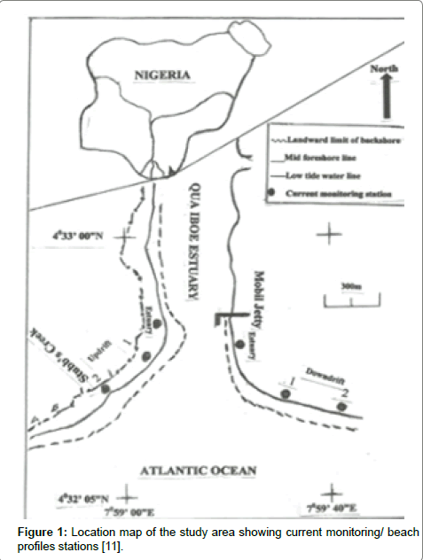
Figure 1: Location map of the study area showing current monitoring/ beach profiles stations [11].

The study covered a period of nine days from September 28, to October 6, 2013. The area was divided into updrift and downdrift shoreline morphologic compartments adjoined to Qua-Iboe estuary respectively (Figure 2). Littoral cell was demarcated along the beach at 500 m away from the estuary mouth at both updrift and downdrift compartments of the ocean shoreline. Six monitoring stations for hydrodynamic processes were established and geo-referenced with GPS: one station, each at the either sides of the estuarine shoreline at 100m away from the estuary mouth; and two stations, each at 200 m and 500 m locations along the downdrift and updrift ocean shoreline from the estuary mouth respectively (Figure 1). At each monitoring station along the ocean shoreline, five geomorphic beach segments were delineated thus: backshore, berm, and upper, mid- and lower foreshore. Beach profiles were made at each station daily over a neapspring tidal phase. Linear beach profile measurements were converted to beach volumetric change within a one-metre wide transect.

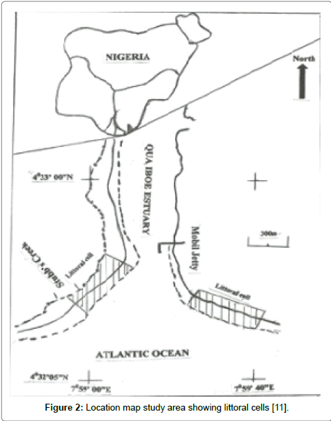
Figure 2: Location map of the study area showing current monitoring/ beach profiles stations [11].

Beach Profile

The cross-shore beach profile surveys at the updrift and downdrift ocean shoreline stations representing neap (28-4-2013), mean (2-10- 2013) and spring (5-10-2013) tide data are presented below:

Beach Sedimentation

The beach sedimentation patterns are considered below under updrift and downdrift volumetric change, shoreline morphology and orientation.

Updrift

i. At station 1 which was closer to the estuary, the net sedimentation pattern fluctuated between 0.72 m³ and -9.6 m³, and the net volumetric change between neap and spring tide was -8.88 m³ (Figure 3).

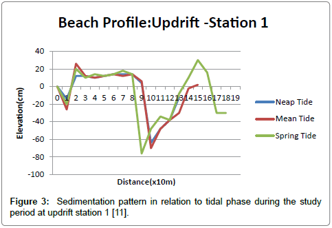
Figure 3: Sedimentation pattern in relation to tidal phase during the study period at updrift station 1 [11].

ii. The beach sedimentation values at station 2 away from the estuary computed between neap and spring tide were 4.2 m³ and -0.3 m³. A net value of 3.9 m³ was recorded (Figure 4).

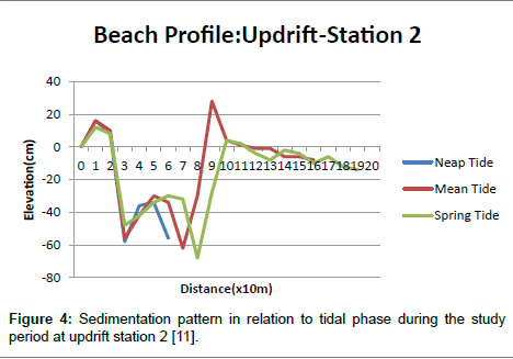
Figure 4: Sedimentation pattern in relation to tidal phase during the study period at updrift station 2 [11].

iii. Station 2 showed accretion while station 1experienced erosion during the study period. However, the net volumetric change of -4.98 m³ indicating erosion was recorded at updrift shoreline stations.

Downdrift

i. The sedimentation pattern at station 1 fluctuated between 39m³ and -8.28 m³. A net volumetric change of 21.72 m³ was recorded between neap and spring tide (Figure 5).

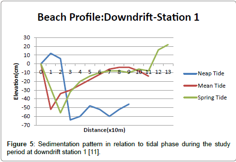
Figure 5: Sedimentation pattern in relation to tidal phase during the study period at downdrift station 1 [11].

ii. Station 2 was characterized by accretion as indicated by sedimentation values of 30 m³ and -10 m³. A net beach volumetric change of 20 m³ was recorded (Figure 6).

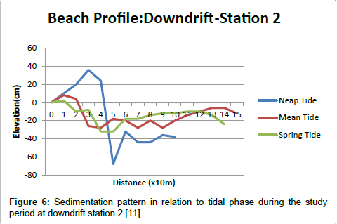
Figure 6: Sedimentation pattern in relation to tidal phase during the study period at downdrift station 2 [11].

• In considering the two stations, the total volumetric change of 40.72 m³ was recorded at the downdrift shoreline stations which indicate sediment accretion.

Sediment Budget Analysis

The quantitative estimate of sediment gains and losses at the littoral cells (Figure 2) and compartments can be determined using sediment base analysis system equation which runs on Windows 95,98 and NT platform [1].

ΣQsource-ΣQsink-ΔV+P-R=Residual (2)

However since the above sediment equation is a computer-based system, new sediment budget equations modified from equation (2) above are developed and applied in this sediment budget analysis thus:

If ΣQsource-ΣQsink = 0 (Equilibrium) (3)

Sediment Budget= 1/5 ( ΣQsource )x t (4)

If ΣQsource-ΣQsink > 0 (surplus)(5)

Sediment Budget = -[ (ΣQsource-ΣQsink) - (Rv x L)]t(6)

If ΣQsource-ΣQsink < 0 (deficit)(7)

Sediment Budget = -[ (ΣQsource-ΣQsink) - (Rv x L)] t=Residual(8)

Where ΣQsource - represents accretion and ΣQsink - represents erosion, Rv- stands for the rate of volumetric change, L- represents the length of littoral cell while t- represents the budget period. The preceding negative sign is a factor which determines the quantity of sediment that can be removed from or placed into the littoral cell. But Rv x L in equation (8) is the sustainability factor which is denoted as Qs. In a sediment budget deficit, the factor- Qs provides a measurable volume of sediment required as a control to the actual sediment volume needed for beach nourishment within a littoral cell. Whereas, in a budget surplus, Qs provides a maximum volume of sediment which can be removed from a littoral cell without upsetting the natural potential of the beach to regain it morpho-dynamic balance in favour of accretion. Therefore equation (8) can equally be written as:

Sediment Budget = -[ (ΣQsource-ΣQsink) - Qs ]t =Residual(9)

Moreover, equation ( 9) can be further expanded as it is applied in this budget analysis thus:

Sediment Budget = -[( [ ΣA(1,2,…)]/n –[ ΣE(1,2,…) ]/n) - (Rv x L)] t=Residual(10)

Where: A=Accretion

B=Erosion

n=Total number of beach profile survey transects

(1,2,..) =Beach profile transects

Sediment budget for updrift beach

Station 1

Accretion (A) =0.72 m³

Erosion (E) =9.6 m³

Volumetric Change = A-E =(0.72-9.6) =-8.88 m³

Station 2

Accretion (A) =4.2 m³

Erosion (E) =0.3 m³

Volumetric Change = A-E= (4.2-0.3)m³ =3.9 m³

Average Volumetric Change for the beach = (ST1+ST2)/2 =(- 8.88+3.9) m³/2

= -4.98m³/ 2=-2.49 m³

The rate of volumetric change per day (Rv) is given as:

(11)

Where: n = number of days.

= -2.49 m³/8-1=-0.356 m³/day (corrected to 3 significant Figures)

Therefore, the rate of volumetric change (Rv) per 1m transect (sublittoral cell) at the beach per day =-0.356 m³/day

Hence, the rate of volumetric change within 500m littoral cell (L) is given as:

(12)

ΣQsink = E1+E2 =(0.3+9.6)m³ =9.9 m³

AverageΣQsink =9.9 m³/2 =4.95 m³ per 1 m sub-littoral transect per day

ΣQsink for 500 m littoral cell per day is given as:

(13)

ΣQsink =2475m³

ΣQsource =A1+ A2=0.72 m³+3.9 m³= 4.62 m³

Average ΣQsource = 4.62 m³/2= 2.31m³ per 1m transect of sub littoral cell per day.

ΣQsource for 500m littoral cell is given as:

(14)

ΣQsource for 500 m littoral cell per day =1155 m³

Therefore ΣQsource-ΣQsink =(1155-2475)m³ = -1320 m³ per day (Deficit)

Budget Estimate =-[ (ΣQsource-ΣQsink) - (Rv x 500)]t (15)

= -[(-1320-178) m³]t

= -[-1498 m³]t

=[1498 m³]t

Where: t = 1 day;

The volume of sediment which can be added to the beach to offset the rate of erosion per day is1498m³

Where t = 1 year (365 days);

Therefore sediment budget estimate for sediment supply to offset the rate of erosion at the littoral cell per a year is given as:

1498 m³ x 365 =546770 m³ per year

Sediment Budget for downdrift beach

Station 1

Accretion (A) =39 m³

Erosion (E) =8.28 m³

Volumetric Change = A-E =(39-8.28 m³) = 21.72 m³

Station 2

Accretion =30 m³

Erosion =10 m³

Volumetric Change = A-E= (30-10) m³ =20 m³

Average Volumetric Change for the beach =(ST1+ST2)/2 =(21.72+20) m³/2

= 41.72 m³/ 2= 20.86 m³

The rate of volumetric change per day(Rv) is given as:

(16)

Where: n=number of days

= 20.86 m³/8-1= 2.98 m³/day(corrected to 3 significant Figures)

Therefore, the rate of volumetric change (Rv) per 1m transect (sublittoral cell) at the beach per day = 2.98 m³/day

Hence, the rate of volumetric change within 500 m littoral cell (L) is given as:

(17)

ΣQsink = E1+E2 =(8.28+10) m³ =18.28 m³

AverageΣQsink =18.28 m³/2 =9.14 m³ per 1 m sub littoral transect per day

ΣQsink for 500m littoral cell per day is given as:

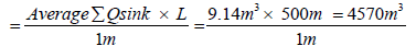(18)

ΣQsink =4570 m³

ΣQsource =A1+ A2=39 m³+30 m³= 69 m³

Average ΣQsource = 69 m³/2= 34.5 m³ per 1m transect of sub littoral cell per day.

ΣQsource for 500 m littoral cell is given as:

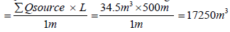(19)

ΣQsource for 500 m littoral cell per day =17250 m³

Therefore ΣQsource-ΣQsink =(17250-4570) m³ = 12680 m³ per day (Surplus)

Budget Estimate =-[ (ΣQsource-ΣQsink) - (Rv x 500)]t (20)

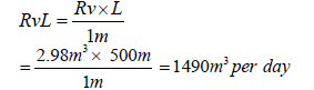
= -[(12680-1490) m³]t

= -[11190 m³]t

=-[11190 m³]t

Where t =1 day

The volume of sediment which can be removed from the beach without erosion per day is 11190 m³ .

Where t = 1 year (365 days);

The sediment budget estimate for the littoral cell per a year is given as: -11190 m³ x 365 = -4084350 m³ per year.

Hence, the volume of sediment which can be removed from the littoral cell for a year is 4084350 m³.

Therefore, sediment budget estimate for the two beaches reveals sediment deficit at the updrift beach and surplus at the downdrift. The sediment budget deficit at the updrift beach is an indication of erosion when compared with the budget surplus at the downdrift which showed accretion. From the budget analysis, the rate of deposition at the downdrift is 8.37 times higher than the rate of erosion (178 m³/day) in a littoral cell at the updrift. This implies that the effect of wave processes which are responsible for erosion at the area is drastically reduced perhaps towards the commencement of another cycle of deposition. On the other hand, the high rate of accretion (1490 m³/day ) at sublittoral cell at the downdrift can be attributed to sediment transport from the updrift beach through the surf-zone across the estuary due to storm surge incident at the shoreline in 2011 (Udo-Akuaibit, 2013). It is from these sedimentary deposits that flood tidal currents, in recent times, transported and rebuilt the downdrift shoreline which result in sediment budget surplus.

It is therefore instructive by the above analysis that the updrift shoreline is threatened by severe erosion and would require much fund to design and establish a control system unlike the downdrift counterpart which has a sediment budget surplus.

The knowledge of sediment budget analysis was noted as an indispensable tool for a successful design and implementation of coastal defence structure and management. It was also found, despite the uncertainties associated with field measurements, as a dependable source of information in decision making for shoreline protection and management by coastal zone managers and coastal engineers. Besides, the new sediment budget equation was easy and simple to work with using beach profile data.

I wish to thank my Master of Science Degree thesis supervisor Professor A Chidi Ibe of the Institute of Natural Resources, Environment and Sustainable Development, University of Port Harcourt, Rivers State and my co-Supervisor Professor E. E.Antia- Director, National Centre for Marine Geosciences, Nigerian Geological Survey Agency, Yenagoa, Bayelsa State for their inspirations. Additional thanks to Charles Odeh, Theresa Udeh and Kinsley Nwogbidi for their field assistance. Also, I wish to acknowledge the financial support for the thesis by the Mac Arthur Foundation, Chicago, U.S.A. through the Institute of Natural Resources, Environment and Sustainable Development, University of Port Harcourt, Rivers State, Nigeria.