International Journal of Advancements in Technology
Open Access
ISSN: 0976-4860
ISSN: 0976-4860
Review Article - (2018) Volume 9, Issue 4
This paper focuses on developing the physics-based model of the SCR system. Through the use of first principles, governing equations of the SCR physics-based model are achieved. The SCR system is modeled in a series of segments. The main reactions are ammonia adsorption, desorption, reduction, and ammonia oxidation. The resulting non-linear partial differential equations are discretized and linearized to obtain a state space model. The model is extended to a sufficiently large order to achieve accuracy. The developed model is analyzed and the system dynamics are studied, validated using simulation studies of a Urea-SCR system. In addition, reduced order dynamics of the SCR system are also analyzed in this paper.
Keywords: Emission reduction in diesel engines; After-treatment system; SCR; Modelling; Physics based SCR model
Selective Catalytic Reduction (SCR) system is used to reduce the oxides of nitrogen NO and NO2 to N2 and water (H2O). The use of SCR system to reduce NOX emissions has been in place since Engelhard Corporation, in 1957, patented this method in the United States.
SCR technology was implemented on a commercial vehicle to meet the EURO IV regulation. Since then the use of SCR in automotive applications has been increasing. There are other technologies such as EGR (Exhaust Gas Recirculation) and LNT (Lean NOX trap) which are used to reduce the NOX emissions.
The SCR system is popular because the engine can be tuned to operate at a very high efficiency which implies higher flame temperatures without compromising the NOX conversion. There are combinations of EGR+SCR, pure SCR, and pure EGR which have been used in the past. For EURO VI and above emission regulations SCR+EGR and SCR only solution are viable options to reduce NOX without compromising on the engine efficiency. FPT was the first to introduce an SCR only solution. Since then a number of other manufacturers like Scania have opted for the SCR only option [1-8].
SCR stands for selective catalytic reduction. SCR catalysts remove nitrogen oxides (NOX) using a reducing agent ammonia (NH3). An SCR catalyst is used to speed up the reactions and to provide a surface on which the reactions take place. As mentioned earlier the reducing agent is carried on board the vehicle as an aqueous solution containing 32.5% urea. This solution is called AdBlue and is used as the storage and transportation is easier.
The NH3 storage model consists of modeled reaction rates. These reaction rates are used to calculate the gas phase concentrations of NOX as well as NH3. Detailed kinetic models such as the ones used by catalyst manufacturers such as Johnson Matthey and BASF are very detailed. They usually include the reaction rates of all the reactions that occur or certain side reactions that might occur inside an SCR converter.
The chemical kinetics in an SCR system involves the following reactions:
Adsorption and desorption of NH3 onto the surface of the catalytic converter
This mechanism can be depicted by the following reaction:
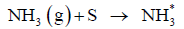 Where S in equation denotes a free site on the surface of the catalytic converter and NH3* denotes an ammonia molecule adsorbed onto the surface of the catalytic converter. A free site on a catalytic surface is an empty void. This is formed due to the adsorbent (the coating of the catalytic converter in this case) not being completely surrounded by the other adsorbent atoms. This empty site is occupied by the ammonia molecules. The forward reaction in the equation denotes adsorption of the ammonia molecule while the reverse denotes desorption of NH3* molecule.
SCR reactions
There are mainly three important chemical reactions that occur between the ammonia stored in the catalyst and the NOX entering the catalyst.
The first SCR reaction is called the standard SCR. This reaction is depicted below:
4 NH3 + 4 NO+O2 → 4 N2 + 6 H2O
In this reaction, gas phase NOX, Oxygen, and adsorbed Ammonia react with each other to produce water and Nitrogen. This reaction occurs dynamically, and the goal of this thesis is to determine a model that captures this conversion accurately, thereby setting the stage for a control design that allows the determination of an optimal profile of the Ammonia input that allows a maximum NOX conversion.
Another important SCR reaction is called the Fast SCR. This reaction is depicted below:
4 NH3 + 2 NO+ 2 NO2 →4 N2 + 6 H2O
The above equation consumes one mole of NH3 per mole of NOX and is faster compared to the standard SCR. The Diesel Oxidation Catalyst (DOC) alters the ratio of NO/NO2. The ratio of NO/NO2 in the engine out NOX will thus change after the DOC. This will ensure that a major portion of the NOX gets converted through the fast SCR reaction. The fast SCR is usually the dominant reaction when the ratio of NO/ NO2 is close to one.
The last SCR reaction is called the Slow SCR and is shown below:
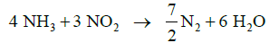
The slow SCR reaction is usually not relevant as it can be neglected. The reaction rate of the slow SCR becomes significant when the entire NO is consumed inside the catalytic converter.
SCR temperature model
The SCR model also consists of a sub-model that calculates the temperature dynamics of the SCR system. The temperature model is based on simple heat balance. The SCR is assumed to be a perfect heat exchanger. This implies that the temperature exhaust gas leaving the SCR is equal to the temperature of the SCR. The SCR is assumed to be very well insulated therefore convective and radiative losses are ignored.
A physical and chemical phenomenon in the catalyst
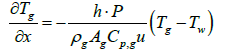
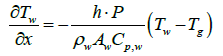
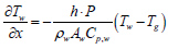
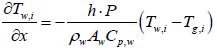
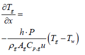
When exhaust gas containing NH3 and NOX is supplied into the channel, several physical and chemical phenomena occur. The first phenomenon is a diffusion of species of NH3 and NOX between flowing gas and stationary gas in the wash coat which is then followed by chemical reactions between molecules on the surface of the catalyst. The third phenomenon is heat transfer between the flowing gas and the wash coat/structure. To model these phenomena, we need at two energy equations for the gas and the wash coat/structure and species equations for each species in the flowing channel, the stationary gas of the wash coat, and on the catalyst. Below are the energy equations to calculate wall temperature and gas temperature (Figure 1).
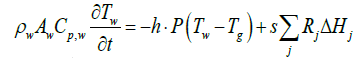
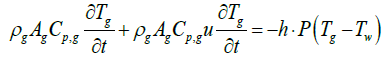

Figure 1: Top view of each channel of the urea-SCR with a honeycomb structure.
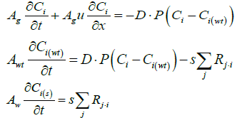
The below equations represent equations of ith species in the flowing gas and the stationary gas in a wash coat, and on the catalyst surface, respectively.
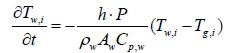
Below are the energy equations of wall and gas, respectively.
 (1)
(1)
 (2)
(2)
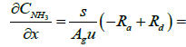
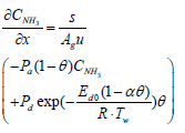
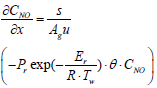
Below are the NH3, and NO species equations of flowing gas in a channel.
 (3)
(3)
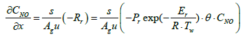 (4)
(4)
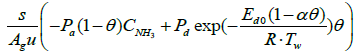
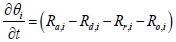
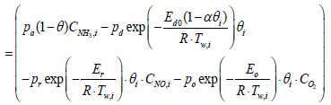
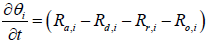
The species equation of adsorbed Ammonia on the surface of the catalyst. θ is the fraction loading of Ammonia onto the catalyst and defined by  in which Ω is the number of reaction-sites per volume of wash coat (Figure 2).
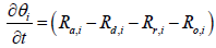
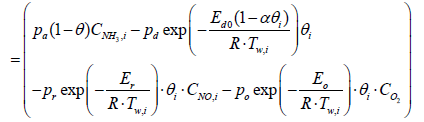 (5)
(5)

Figure 2: Schematic of a sample-size reactor experiments.
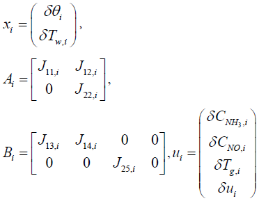
To derive state space form for the whole system, we first discretized equations in the spatial domain, and derived state space form equation for governing equations which are continuous in time for each segment. Then, every state equation for each segment is assembled into one large state space equation (Figure 3).

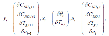
Figure 3: Inputs, outputs, and state variables of each segment.
Discretization in space
To derive the reactor's state space equation, the reactor is first discretized in the axial direction as in Figure 3 in which inputs, output, and state variables for a segment are shown. Equations (3), (4), and (5) that pertain to spatial derivates are discretized spatially, but governing equations (1) and (2) are still in the continuous form after discretization.
Equations (3), (4), and (5) which are governing equations for CNH3, CNO, and Tg are discretized in the axial direction (x-direction in the equations). In this procedure, the state variables, and Two,i are assumed to be constant in each segment.
Using the first-order implicit Euler method, gas temperature output of ith segment can be expressed as
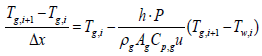 (6)
(6)
Where, subscription i, is an index for segmentation, and state variable Tw,i, is assumed to be a constant in the ith segment. Therefore, gas temperature output of ith segment is expressed as follows:
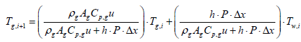 (7)
(7)
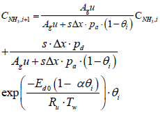
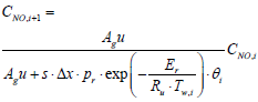
Similarly, a discretized form of the species equations of gas-phase Ammonia and Nitrogen Monoxide (equations 3 and 4) are expressed as
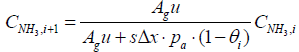
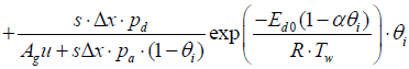 (8)
(8)

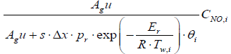 (9)
(9)
Equations 2 and 5 after discretization, are expressed as
 (10)
(10)
 (11)
(11)
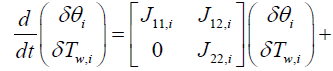
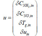
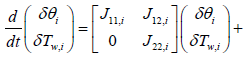
Next step is to linearize the five governing equations, two of which are continuous in time domain and three of which are discretized in the space, around an equilibrium point that is determined using nominal input conditions. The equilibrium point for each segment i is determined by CNH3,i,eq, CNO,i,eq, θi,eq , Tw,i,eq , Tg,i,eq , and ui,eq .These, in turn, are determined by supplying a constant CNH3,in , CNO,in , Tg,in and uin,eq with the resulting steady-state values of the ith segment set as the corresponding equilibrium point. Using these equilibrium points, Equations (10) and (11) can be linearized around equilibrium points as follows:
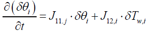
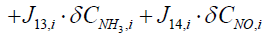 (12)
(12)
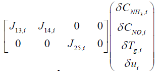
 (13)
(13)
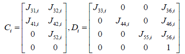
where Jkl,i means that partial derivative of a k'th index variable with respect to i'th index variable under equilibrium in i'th segment Variables indexed by k and l include the following: (Table 1).
1: θ
2: Tw
3: CNH3
4: CNO
5: Tg
6: u
| Before Discretization for the whole reactor | After Discretization for each segment |
|---|---|
 |
 |
 |
 |
 |
 |
 |
 |
 |
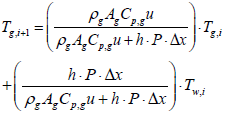 |
Table 1:Governing equations before and after discretization.
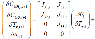
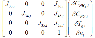
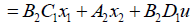
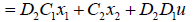
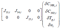
From Equations (12) and (13), system matrix for the i'th segment can be expressed as follows:
 (14)
(14)
This is in turn, 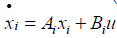 (15)
(15)
Where,
In order to obtain the output equation for the i'th segment, governing Equations (8), (9), and (7) should be linearized around equilibrium point as follows:
 (16)
(16)

 (17)
(17)
 (18)
(18)
The output equations can be summarized from equations (16), (17), and (18) as follows:
 (19)
(19)
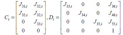
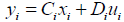
This is, in turn, expressed compactly as:
yi = Cixi + Diu (20)
Where,
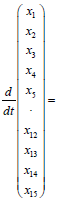
After we first carried out a discretization and linearization procedure to convert the nonlinear PDEs into the linear system, we assembled state space equations for each segment into a single, large, state space equation. External inputs include CNH, CNO,in, Tg.in, and uin , the inputs to the first segment, while system outputs are the outputs of the N'th segment, and are denoted as CNH,out, CNO,out and Tg,out. Gas velocity is assumed to be uniform for the sake of simplicity. It was observed that a choice of N=15 resulted in sufficient accuracy, leading to a 30th order linear system (Figure 4).

Figure 4: Discretization of a catalyst block, input and output variables, and state variables.
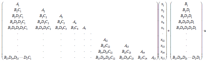
First we placed every state space equation into one state space equations as follows:
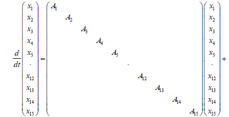
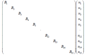 (21)
(21)
Because every segment is connected by input and output, Equation (21) can be expressed in terms of the system input
And, state variables up to the ith segment instead of ui. For example, the second segment's state space equation is expressed as follows:

 (22)
(22)
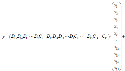
The output matrix of the second segment can be also expressed by system input and state variables as follows:

Equation (23) summarizes (15) and (20) into one large state space equation that includes 15 state space equations for 15 segments.
 (23)
(23)
 (24)
(24)
Where,

Analysis of the developed physics-based model is carried out in this section. It involves computing the state space model for one individual segment of the catalyst block and extending the same to 30th order linear system for sufficient accuracy.
Reviewing the equations (14) and (15)
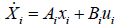
System and input matrices A, B can be expressed as
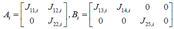
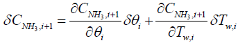
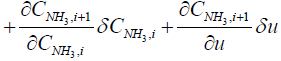
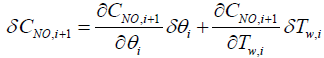
From the equations (19) and (20)
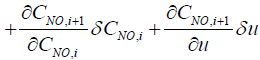
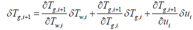
i+1th values which correspond to CNH3,i+1, CNO,i+1 and Tg,i+1 are computed by the following equations:
The state variables Tw,i and θi are assumed to be constant in each segment.
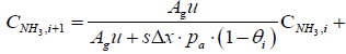
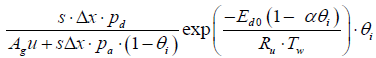
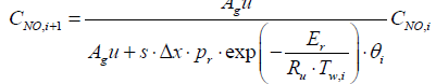
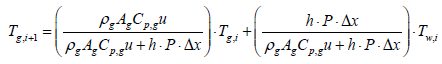
Substituting the parameters in the above equations will give
CNH3,i+1 = 0.907 CNH3,i + 6.9615 × 10⁻¹⁵
CNO,i+1 = 0.9999 CNO,i
Tg,i+1 = 0.632 Tg,i + 183.2
The concentration of Ammonia and Nitrogen oxide in ppm is 330.
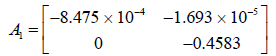
Analyzing the dynamics of a segment
The system matrix A1 is computed from the Jacobians associated with it (Tables 2 and 3).
| J11,i | -0.25 CNH3,i - 6.46 × 10⁻⁴ |
| J12,i | -0.0208 CNO,i -6.153 × 10⁻⁸ |
| J22,i | -0.4583 |
| J13,i | 0.2498 |
| J14,i | -4.264 × 10⁻⁴ |
| J25,i | 0.4583 |
| J31,i | 0.0845 CNH3,i + 3.986 × 10⁻⁴ |
| J32,i | 4.31 × 10⁻¹¹ |
| J41,i | -1.17 × 10⁻¹³ CNO,i |
| J42,i | -2.73 × 10⁻¹⁸ CNO,i |
| J33,i | 0.907 |
| J52,i | 0.36787 |
| J44,i | 0.9998 |
| J55,i | 0.632 |
| J36,i | 2.516 CNH3,i -1.85 × 10⁻⁸ |
| J46,i | 0.0024 CNO,i |
| J56,i | 0.632 |
| J66,i | 1 |
Table 2: Jacobians associated with the state space equations with practical parameters.
| CNH3, in | 8.11 × 10⁻⁴ |
| CNO,in | 8.11 × 10⁻⁴ |
| CO2 ,in | 1.96616 |
Table 3: Concentrations NH3, NO, and O2 at the input.
The Eigen values of A1 are observed to be -0.00084 and -0.4583.
Both the poles of the system matrix corresponding to A1 are on the right side of the s-plane and the system is stable.
Analyzing the system -30th order linear model
The non-linear model is linearized to obtain the 30th order model computed from the equations 19, 20 with, CNO,i and Tg,i values regularly updated for each segment starting from input to the output.
The MATLAB code to compute the 30th order system matrix is listed in the Appendix section. The Eigen values for the system are found to be -Eigen values of A30 × 30 system matrix- [-0.000697 -0.000702 -0.000709 -0.000715 -0.000722 -0.000730 -0.000734 -0.000745 -0.000756 -0.000770 -0.000783 -0.000797 -0.000812 -0.000829 -0.000848 -0.4583 -0.4583 -0.4583 -0.4583 -0.4583 -0.4583 -0.4583 -0.4583 -0.4583 -0.4583 -0.4583 -0.4583 -0.4583 -0.4583 -0.4583].
It can be observed that the all the 30 poles are real and negative. The poles are placed in the negative half of the s-plane. The system is stable (Figure 5).

Figure 5: The Eigen values plot A30 × 30.
From the Eigen values plot, we can observe that the poles of the system are repetitive and many of them are almost closely placed. This also means that the system order can be reduced preserving the dynamics of the original system.
Reduced order system dynamics
Reducing the main interface to model approximation algorithms.
Reducing the 30th order linear model into 10th order using Hankel SV model reduction [27]. Hankel singular values of a stable system indicate the respective state energy of the system. Hence, the reduced order can be directly determined by examining the system Hankel SV's. Model reduction routines, which based on Hankel singular values are grouped by their error bound types. In many cases, the additive error method GRED=reduce (G, ORDER) [in MATLAB] is adequate to provide a good reduced order model which reduces the relative errors between G and GRED tends to produce a better fit.
In this paper, the order of the system is reduced to 10 to analyze its dynamics in that order.
Eigen values: [-0.4211+0.1614i, -0.4211-0.1614i, -0.3583+0.1126i, -0.3583-0.1126i, -0.3278+0.0569i, -0.3278-0.0569i, -0.3186, -0.00052, -0.00058+0.000154i, -0.00058+0.000154i] (Figures 6-10).

Figure 6: The Eigen values plot A10 × 10.

Figure 7: SIMULINK model for the state space equation of order 30 (step change of 10 ppm).

Figure 8: Response of the 30th order model 10 ppm change in Ammonia.

Figure 9: The SIMULINK model for the reduced state space equation (step change of 10 ppm).

Figure 10: Response of the 10th order model 10 ppm change in Ammonia.
Output comparison of the 30th order and the reduced 10th order models: The outputs of both the 30th order and 15th order systems are analyzed for a step change of 10 ppm in the concentration of Ammonia while all the other parameters remain same.
From both the above plots (in Figures 7 and 9) it is reasonably inferred that the response of the reduced order model is similar to the original 30th order model. The steady state output values of NH3 in both responses are nearly the same. For a sufficiently higher model, the dynamics of the reduced order model is expected to be the same as the higher order model with minimum errors.
Nonlinear models are derived based on physical and chemical interpretation of the catalyst and certain simplifications. We subsequently discretized and linearized the nonlinear equations and analyzed the system dynamics of the catalyst. The following are some of our main observations regarding the SCR dynamic model:
• The steady state output of the first principle-based model given sufficiently accurate results for a higher order linear system. Order of 30 is chosen for satisfactory accuracy in results
• The dynamics of the reduced order system is the same as the higher order linear model. Since many poles are repetitive, the system can be reduced to a degree which gives an almost the same response as the higher order model also keeping in view of the errors involved in the reduction method. Dynamics of settling time and trend are seen to be the same for both the models
• Although the model of the SCR developed during this thesis was for an extruded Vanadia formulation, the SCR model can be easily applied to other catalyst formulations e.g. Copper-Zeolite. This would, however, require that tests be conducted on the chosen formulations to identify the significant chemical kinetics. The model offers flexibility to model additional reactions or remove unnecessary reaction kinetics.
I wholeheartedly thank Dr. M Umapathy, Professor, Instrumentation and Control Engineering, NIT Trichy., for his constant support and guidance, and without whom the completion of this project in fruition would not have been possible.